5. Software Architecture

This section describes the overall software architecture (Section 5.1), the coupling of Modelica with EnergyPlus (Section 5.2), the integration of the QSS solver with OPTIMICA (Section 5.4), and the OpenStudio integration (Section 5.5).

5.1. Overall software architecture

Fig. 5.1 shows the overall software architecture of SOEP.

The Application on top of the figure may be an equipment sales tool that uses an open, or a proprietary, Modelica model library of their product line, which allows a sales person to test and size equipment for a particular customer.

The HVAC Systems Editor allows drag and drop of components, which are read dynamically from the Modelica Library AST, similar to what can be done in today’s OS schematic editor. In contrast, the Schematic Editor allows to freely place and graphically connect Modelica components. Once models have been manipulated in the Schematic Editor, OS can only simulate them, but not apply OS Measures to it, as models may have become incompatible with the OS Measures. (This could in the future be changed by parsing the AST of the model.)

In the Schematic Editor, user-provided Modelica libraries can be loaded (for example, if a company has their own control sequence library), manipulated and stored again in the user-provided Modelica library. This functionality is also needed for the OpenBuildingControl project.

Currently, the OpenStudio Model Library is compiled C++ code. Our integration will generate a representation of the Modelica library that allows OpenStudio to dynamic load models for the SOEP mode.

Fig. 5.1 : Overall software architecture.

5.2. Coupling of EnergyPlus with Modelica

This section describes the coupling of EnergyPlus with Modelica. The coupling allows two types of interactions between the two tools:

1. The EnergyPlus envelope model can be coupled with the Modelica room model, which in turn is coupled to Modelica HVAC and interzone air exchange. This is described in Section 5.2.3.1.

2. Modelica can instantiate and then read EnergyPlus output variables. This is described in Section 5.2.3.4.

3. Modelica can instantiate and then set the values of EnergyPlus schedules and EMS actuators. This is described in Section 5.2.3.5.

Users will set up this data exchange by instantiating corresponding Modelica models or blocks. These Modelica instances will then communicate with EnergyPlus, using Modelica C functions, to package EnergyPlus as an FMU for Model Exchange 2.0. Modelica will then automatically instantiate this FMU and use it for the simulation using the FMI Library from Modelon.

5.2.1. Assumptions and limitations

To implement the coupling, will make the following assumptions:

1. Only the lumped room air model will be refactored, not the room model with stratified room air. The reason is to keep focus and make progress before increasing complexity.

2. The HVAC and the pressure driven air exchange (airflow network) are either in Modelica or EnergyPlus. The two methods cannot be combined. The reason is that the legacy EnergyPlus computes in its “predictor/corrector” the room temperature as follows:

   1. First it computes the HVAC power required to meet the temperature set point,

   2. next it simulates the HVAC system to see whether it can meet this load, and

   3. finally it updates the room temperature using the HVAC power from step (b).

   This is fundamentally different from the ODE solver used by SOEP who sets the new room temperature and time, computes the time derivative, and then recomputes the new time step.

3. In each room, mass, as opposed to volume, is conserved. The reason is that this does not induce an air flow in the HVAC system if the room temperature changes. Hence, it decouples the thermal and the mass balance.

5.2.2. Unit system

Modelica and EnergyPlus each have their own unit system. Spawn of EnergyPlus will automatically convert between these units, using information from the modelDescription.xml file, or stop the simulation if an unknown unit is encountered. The Modelica Buildings Library will do the unit conversion using C functions. These C functions will convert between the units shown in Table 5.1. The table also shows unit strings that are allowed to use by EnergyPlus to tell Modelica the unit of the exchanged inputs and outputs. The C functions will then convert the quantity as needed to represent it in the units shown in the column Modelica Unit.

Table 5.1 Unit specification of EnergyPlus I/O.

Quantity	EnergyPlus Unit String	Modelica Unit
Angle (rad)	rad	rad
Angle (deg)	deg	rad
Energy	J	J
Illuminance	lux	lm/m2
Humidity (absolute)	kgWater/kgDryAir	1 (converted to mass fraction per total mass of moist air)
Humidity (relative)	%	1
Luminous flux	lum	cd.sr
Mass flow rate	kg/s	kg/s
Power	W	W
Pressure	Pa	Pa
Status (e.g., rain)	(no character)	1
Temperature	degC	K
Time	s	s
Transmittance, reflectance, and absorptance	(no character, specified as a value between 0 and 1)	1
Volume flow rate	m3/s	m3/s

5.2.3. Partitioning of the models

To link EnergyPlus and Modelica, the models are partitioned as shown in as shown in Fig. 5.2. Loosely speaking, everything that is air and controls is simulated in Modelica, while EnergyPlus simulates heat conduction in solid and through windows. Both simulators can declare and use schedules, and they can interact through the thermal zone model, through EnergyPlus outputs and through EnergyPlus schedules and EMS actuators.

Fig. 5.2 : Partitioning of the envelope, room and HVAC model.

The following Section 5.2.3.1 specifies the coupling of these models, Section 5.2.4 describes the API used to generate the FMU, and Section 5.2.5 describes the synchronization of the tools.

5.2.3.1. Coupling of the envelope model

To couple the Modelica room model to the EnergyPlus envelope model, EnergyPlus exposes the following parameters. Modelica will obtain their values during the initialization of the Modelica model.

Variable	Quantity	Unit
V	Volume of the zone air.	m3
AFlo	Floor area of the zone.	m2
mSenFac	Factor for scaling the sensible thermal mass of the zone air volume.	1

The following time-dependent variables are exchanged between EnergyPlus and Modelica during the time integration for each thermal zone.

Variable	Quantity	Unit
From Modelica to EnergyPlus
T	Temperature of the zone air.	degC
X	Water vapor mass fraction per total air mass of the zone.	kg/kg
mInlets_flow	Sum of positive mass flow rates into the zone for all air inlets (including infiltration).	kg/s
TInlet	Average of inlets medium temperatures carried by the mass flow rates.	degC
QGaiRad_flow	Radiative sensible heat gain added to the zone.	W
t	Model time at which the above inputs are valid, with \(t=0\) defined as January 1, 0 am local time, and with no correction for daylight savings time.	s
From EnergyPlus to Modelica
TRad	Average radiative temperature in the room.	degC
QConSen_flow	Convective sensible heat added to the zone, e.g., from surface convection and from the EnergyPlus’ People or Equipment schedule.	W
QLat_flow	Latent heat gain added to the zone, e.g., from mass transfer with moisture buffering material and from EnergyPlus’ People schedule.	W
QPeo_flow	Heat gain due to people (only to be used to optionally compute CO2 emitted by people).	W
nextEventTime	Model time \(t\) when EnergyPlus needs to be called next (typically the next zone time step).	s

Note that the EnergyPlus object ZoneAirContaminantBalance either allows CO2 concentration modeling, or a generic contaminant modeling (such as from material outgasing), or no contaminant modeling, or both. To avoid ambiguities regarding what contaminant is being modeled, we do not receive the contaminant emission from EnergyPlus. Instead, we obtain the heat gain due to people, which is then used to optionally compute the CO2 emitted by people.

The calling sequences of the functions that send data to EnergyPlus and read data from EnergyPlus is as for any continuous-time variable in FMI. That is, at any time instant, variables can be set multiple times, and the values returned by EnergyPlus must be computed using the current input variables. (For example, multiple calls within a time step are used to compute the derivative of QConSen_flow with respect to T.)

5.2.3.2. Coupling of an opaque construction

The following interface models the coupling of an heat transfer model for an opaque construction with the two surfaces of an EnergyPlus BuildingSurface:Detailed. This allows for example coupling of a radiant slab that is modeled in Modelica to the EnergyPlus thermal zone model. Examples of such radiant systems include a floor slab with embedded pipes and a radiant cooling panel that is suspended from a ceiling.

The partitioning is such that Modelica models the heat transfer between the surfaces and the device behind the surface (e.g., a concrete slab with pipes or a radiant panel) and sends the surface temperatures to EnergyPlus. EnergyPlus models the heat transfer between the front surface and its respective thermal zone, and it models the heat transfer of the back surface and its respective boundary condition, which could be another thermal zone, the outside, or the ground coupling, depending on its specification of the Outside Boundary Condition in EnergyPlus. Therefore, EnergyPlus will model all heat that enters the surface from its external boundary condition. For a thermal zone or the outside, this is the convective heat transfer, the short-wave radiation absorbed by the surface and the long-wave radiation absorbed minus emitted by the surface. For ground coupled surfaces, this is the heat transfer from the ground.

EnergyPlus exposes the following parameter, which Modelica will obtain during the initialization.

Variable	Quantity	Unit
A	Area of the surface that is exposed to the thermal zone.	m2

The following time-dependent variables are exchanged between EnergyPlus and Modelica during the time integratione.

Variable	Quantity	Unit
From Modelica to EnergyPlus
TFront	Temperature of the front-facing surface.	degC
TBack	Temperature of the back-facing surface.	degC
t	Model time at which the above inputs T is valid, with \(t=0\) defined as January 1, 0 am local time, and with no correction for daylight savings time.	s
From EnergyPlus to Modelica
QFront_flow	Net heat flow rate from the thermal zone to the front-facing surface, consisting of convective heat flow, absorbed solar radiation, absorbed infrared radiation minus emitted infrared radiation.	W
QBack_flow	Net heat flow rate to the back-facing surface. If coupled to another thermal zone or the outside, this consist of convective heat flow, absorbed solar radiation, absorbed infrared radiation minus emitted infrared radiation. If coupled to the ground, this consists of the heat flow rate from the ground.	W
nextEventTime	Model time \(t\) when EnergyPlus needs to be called next (typically the next zone time step).	s

The calling sequences of the functions that send data to EnergyPlus and read data from EnergyPlus is as for any continuous-time variable in FMI. That is, at any time instant, variables can be set multiple times, and the values returned by EnergyPlus must be computed using the current input variables. (For example, multiple calls within a time step may be used to compute the derivative of QFront_flow with respect to TFront, and QBack_flow with respect to TBack.)

5.2.3.3. Coupling of a zone surface

The following interface models the heat transfer of a surface with the EnergyPlus thermal zone. This allows for example coupling of a radiant heating in the 1st floor that is modeled in Modelica to the EnergyPlus thermal zone model for heat exchange with the zone, while simulating the ground coupling of the slab in Modelica. EnergyPlus models the heat transfer between the surface and the thermal zone. Therefore, EnergyPlus will model the convective heat transfer, the short-wave radiation absorbed by the surface and the long-wave radiation absorbed minus emitted by the surface.

EnergyPlus exposes the following parameter, which Modelica will obtain during the initialization.

Variable	Quantity	Unit
A	Area of the surface that is exposed to the thermal zone.	m2

The following time-dependent variables are exchanged between EnergyPlus and Modelica during the time integratione.

Variable	Quantity	Unit
From Modelica to EnergyPlus
T	Temperature of the surface.	degC
t	Model time at which the above inputs T is valid, with \(t=0\) defined as January 1, 0 am local time, and with no correction for daylight savings time.	s
From EnergyPlus to Modelica
Q_flow	Net heat flow rate from the thermal zone to the surface, consisting of convective heat flow, absorbed solar radiation, absorbed infrared radiation minus emitted infrared radiation.	W
nextEventTime	Model time \(t\) when EnergyPlus needs to be called next (typically the next zone time step).	s

The calling sequences of the functions that send data to EnergyPlus and read data from EnergyPlus is as for any continuous-time variable in FMI. That is, at any time instant, variables can be set multiple times, and the values returned by EnergyPlus must be computed using the current input variables. (For example, multiple calls within a time step may be used to compute the derivative of Q_flow with respect to T.)

5.2.3.4. Retrieving output variables from EnergyPlus

This section describes how to retrieve in Modelica values from the EnergyPlus object Output:Variable.

There will be a Modelica block called EnergyPlus.OutputVariable with parameters

Name	Comment
key	EnergyPlus key of the output variable
name	EnergyPlus name of the output variable as in the EnergyPlus .rdd or .mdd file

At each invocation of the function fmi2GetReal, EnergyPlus will return the output variable that is computed for the current time and all the values set with fmi2SetReal. During the initialization, EnergyPlus will return an initial value.

For Modelica, reading variables will be done using a block with no input and one output.

We assume that these variables are discrete-time variables and hence change their values only at events. Specifically, if \(y(\cdot)\) is a variable of time that is computed in EnergyPlus that is sampled at some time instant \(t\), then Modelica will retrieve \(y(t^+)\), where \(t^+ = (\lim_{\epsilon \to 0} (t+\epsilon), t_{I_{max}})\) and \(I_{max}\) is the largest occurring integer of superdense time.

The Modelica pseudo-code is

when {initial(), time >= pre(tNext)} then
  (y, tNext) = readFromEnergyPlus(adapter, time);
end when;

where adapter stores the data structure used to communicate with EnergyPlus.

5.2.3.5. Sending input to EnergyPlus

This section describes how to send Modelica values to the EnergyPlus objects

1. ExternalInterface:FunctionalMockupUnitExport:To:Schedule, and

2. ExternalInterface:FunctionalMockupUnitExport:To:Actuator.

For reference, examples of instances in EnergyPlus for these objects are as follows.

ExternalInterface:FunctionalMockupUnitExport:To:Schedule,
  OfficeSensibleGain,                           !- EnergyPlus Schedule Name
  Any Number,                                   !- Schedule Type Limits Names
  QSensible,                                    !- FMU Variable Name
  0;                                            !- Initial Value

ExternalInterface:FunctionalMockupUnitExport:To:Actuator,
  Zn001_Wall001_Win001_Shading_Deploy_Status,   !- EnergyPlus Variable Name
  Zn001:Wall001:Win001,                         !- Actuated Component Unique Name
  Window Shading Control,                       !- Actuated Component Type
  Control Status,                               !- Actuated Component Control Type
  yShade,                                       !- FMU Variable Name
  6;                                            !- Initial Value

For the Modelica coupling, these objects need not be declared in the idf file.

For Modelica, exchanging variables with these objects will be done using a Modelica block that has only one input and no output.

As in Section 5.2.3.4, we assume that these variables are discrete-time variables and hence change their values only at events. Specifically, if \(u(\cdot)\) is a variable of time that is computed in Modelica that is sampled at some time instant \(t\), then Modelica will send \(u(\mathbin{^-t})\), where \(\mathbin{^-t} = (\lim_{\epsilon \to 0} (t-\epsilon), 0)\).

With this construct, there is no iteration needed if a control loop is closed between Modelica and EnergyPlus that uses outputs from Section 5.2.3.4 and inputs from this section. To see this, consider a controller in Modelica that will send a control signal \(u(t)\) to EnergyPlus and retrieve from EnergyPlus a measured quantity \(y(t)\). A specific example is a PI controller in Modelica that actuates the shade slat angle in EnergyPlus based on indoor illuminance reported by EnergyPlus. Then, at the time instant \(t\), Modelica will send \(u(\mathbin{^-t})\) and it will retrieve \(y(t^+)\). Hence, no iteration across the tools is required. At the next sample time, Modelica will send the updated control signal that depends on \(y(t^+)\) to EnergyPlus. This simple example also illustrates that inputs and outputs may need for certain applications be exchanged at a sampling rate that is below the EnergyPlus zone time step in order to get satisfactory closed loop control performance.

5.2.3.5.1. Schedules

There will be a Modelica block called EnergyPlus.Schedule with parameters

Name	Comment
name	Name of an EnergyPlus schedule.
unit	Unit of the variable used as input to this block (consistent with column Modelica unit in Table 5.1 )
useSamplePeriod	If true, sample at zone time step and at sample period
samplePeriod	Sample period of component (used if useSamplePeriod = true.

Note

As EnergyPlus has no notion of real versus integer (or boolean) variables, values will be sent as doubles.

The Modelica pseudo-code is

when sample(t0, samplePeriod) then
   sendScheduleToEnergyPlus(pre(u), adapter);
end when;

where t0 is the start of the simulation, samplePeriod is the sample period if this block, and pre(u) is the value of the input before sample(t0, samplePeriod) becomes true.

5.2.3.5.2. Actuators

There will be a Modelica block called EnergyPlus.Actuator with parameters

Name	Comment
variableName	Name of the EnergyPlus variable.
unit	Unit of the variable used as input to this block (consistent with column Modelica unit in Table 5.1 )
componentName	Name of the actuated component unique name.
componentType	Actuated comonent type.
controlType	Actuated component control type.
useSamplePeriod	If true, sample at zone time step and at sample period
samplePeriod	Sample period of component (used if useSamplePeriod = true.

Todo

Why is the Variable name needed? Should this be left out?

No entry in the idf file is required to write to an EMS actuator.

The Modelica pseudo-code is

when sample(t0, samplePeriod) then
   sendActuatorToEnergyPlus(pre(u), adapter);
end when;

where pre(u) is the value of the input before sample(t0, samplePeriod) becomes true.

5.2.4. API used to Export EnergyPlus as an FMU

To export EnergyPlus as an FMU for model exchange, EnergyPlus provides an executable that reads a json configuration file and packages EnergyPlus as an FMU for Model Exchange 2.0.

Note

In the current implementation, we assume that EnergyPlus does not support roll back in time. This will otherwise require EnergyPlus to be able to save and restore its complete internal state. This internal state consists especially of the values of the continuous-time states, iteration variables, parameter values, input values, delay buffers, file identifiers and internal status information. This limitation is indicated in the model description file with the capability flag canGetAndSetFMUstate being set to false. If this capability were supported, then EnergyPlus could be used with ODE solvers which can reject and repeat steps. Rejecting steps is needed by ODE solvers such as DASSL or even Euler with step size control (but not for QSS) as they may reject a step size if the error is too large. Also, rejecting steps is needed to identify state events (but not for QSS solvers).

5.2.4.1. Instantiation

To instantiate EnergyPlus, EnergyPlus generates an FMU 2.0 for model exchange. This is initiated by Modelica, which invokes a system command of the form

spawn path_to_json

where spawn is a program provided by EnergyPlus, and path_to_json is the absolute path of the json file ModelicaBuildingsEnergyPlus.json that configures EnergyPlus. For the case of a model with one thermal zone, the content of this file looks as follows:

{
 "version": "0.1",
 "EnergyPlus": {
   "idf": "/tmp/tmp-spawn/jm_tmpPVJfHP/resources/0/RefBldgSmallOfficeNew2004_Chicago.idf",
   "idd": "/tmp/tmp-spawn/jm_tmpPVJfHP/resources/2/Energy+.idd",
   "weather": "/tmp/tmp-spawn/jm_tmpPVJfHP/resources/1/USA_IL_Chicago-OHare.Intl.AP.725300_TMY3.epw"
 },
 "fmu": {
     "name": "/mnt/shared/modelica-buildings/tmp-eplus-fmuName/fmuName.fmu",
     "version": "2.0",
     "kind"   : "ME"
 },
 "model": {
     "zones": [
         { "name": "office" }
     ]
   }
 }

Using this information, EnergyPlus creates the FMU with name /mnt/shared/modelica-buildings/tmp-eplus-fmuName/fmuName.fmu

We will now describe how to the exchanged variables are configured.

5.2.4.1.1. Envelope model

To configure the variables to be exchanged for the envelope model described in Section 5.2.3.1, the following data structures will be used for a building with a zone called basement and a zone called office.

"zones": [
   { "name": "basement" },
   { "name": "office" }
]

In this case, the FMU must have parameters called basement_V, office_V, basement_AFlo etc. inputs called basement_T and office_T and outputs called basement_QConSen_flow and office_QConSen_flow.

5.2.4.1.2. Opaque construction

To configure the variables to be exchanged for an opaque construction that is part of an EnergyPlus thermal zone as described in Section 5.2.3.2, the following data structures will be used for a building with an EnergyPlus surface called north ceiling office and a zone called south ceiling office. (This requires to add a surface object to EnergyPlus, including all information needed by EnergyPlus such as the surface location and its solar and infrared emissivity.)

"buildingSurfaceDetailed": [
   { "name": "north ceiling office" },
   { "name": "south ceiling office" }
]

5.2.4.1.3. Zone surface

To configure the variables to be exchanged for a surface that is part of an EnergyPlus thermal zone as described in Section 5.2.3.3, the following data structures will be used for a building with an EnergyPlus surface called north ceiling office and a zone called south ceiling office. (This requires to add a surface object to EnergyPlus, including all information needed by EnergyPlus such as the surface location and its solar and infrared emissivity.)

"zoneSurfaces": [
   { "name": "north ceiling office" },
   { "name": "south ceiling office" }
]

5.2.4.1.4. Output variables

To configure the data exchange for output variables, as described in Section 5.2.3.4, consider an example where one wants to retrieve the outdoor drybulb temperature from EnergyPlus.

The corresponsding section in the ModelicaBuildingsEnergyPlus.json configuration file is

"model": {
   "outputVariables": [
     {
       "name":    "Site Outdoor Air Drybulb Temperature",
       "key":     "Environment",
       "fmiName": "Environment Site Outdoor Air Drybulb Temperature"
     }
   ]
}

EnergyPlus will then declare in the modelDescription.xml file an output variable with name as shown in outputVariables.fmiName and units consistent with Table 5.1.

5.2.4.1.5. Schedules

To configure the data exchange for schedules, as described in Section 5.2.3.5.1, consider an example where one wants to write to an EnergyPlus schedule called Lights.

The corresponsding section in the ModelicaBuildingsEnergyPlus.json configuration file is

"model": {
   "schedules": [
     {
       "name"    : "Lights",
       "unit"    : "1", // Unit string as shown in column "EnergyPlus Unit String" in the above table
       "fmiName" : "schedule Lights"
     }
   ]
}

EnergyPlus will then declare in the modelDescription.xml file an input variable with name as shown in schedules.fmiName and unit listed in schedules.unit. Modelica will write to this schedule with units shown in the column EnergyPlus Unit String in Table 5.1.

5.2.4.1.6. EMS actuators

To configure the data exchange for schedules, as described in Section 5.2.3.5.2, consider an example where one wants to write to an EnergyPlus schedule called Lights.

The corresponsding section in the ModelicaBuildingsEnergyPlus.json configuration file is

"model": {
   "emsActuators": [
     {
       "name"          : "Zn001_Wall001_Win001_Shading_Deploy_Status",
       "variableName"  : "Zn001:Wall001:Win001",
       "componentType" : "Window Shading Control",
       "controlType"   : "Control Status",
       "unit"          : "1", // Unit string as shown in column "EnergyPlus Unit String" in the above table
       "fmiName"       : "yShade"
     }
   ]
}

EnergyPlus will then declare in the modelDescription.xml file an input variable with name as shown in emsActuators.fmiName and unit listed in emsActuators.unit. Modelica will write to this EMS actuator with units shown in the column EnergyPlus Unit String in Table 5.1.

5.2.5. Time synchronization

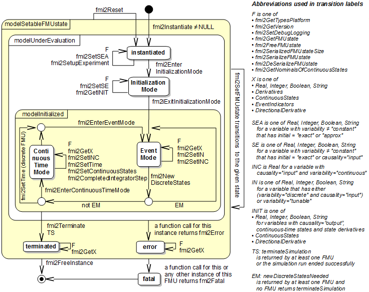
Fig. 5.3 : Calling sequence of Model Exchange C functions in form of an UML 2.0 state machine (Figure reproduced from [MODELISARConsortium14].

Fig. 5.3 shows the state machine for calling an FMU 2.0 for Model Exchange. To communicate with EnergyPlus, we are using the same API and calling sequence. The EnergyPlus envelope model is invoked at a variable time step, using a Modelica time event. In the implementation, EnergyPlus sends the time instant when it needs to be called the next time. Fig. 5.2 shows this as the EnergyPlus time step, but the Modelica implementation allows for any time step requested by EnergyPlus. Therefore, for the envelope model, data is exchanged within the mode labelled Continuous Time Mode in Fig. 5.3. Internally, EnergyPlus samples its heat conduction model at the envelope time step \(\Delta t_z\). EnergyPlus needs to report this to the FMI interface. To report such time events, the FMI interface uses a C structure called fmi2EventInfo which is implemented as follows:

typedef struct{
  fmi2Boolean newDiscreteStatesNeeded;
  fmi2Boolean terminateSimulation;
  fmi2Boolean nominalsOfContinuousStatesChanged;
  fmi2Boolean valuesOfContinuousStatesChanged;
  fmi2Boolean nextEventTimeDefined;
  fmi2Real
  nextEventTime; // next event if nextEventTimeDefined=fmi2True
  } fmi2EventInfo;

The variable nextEventTime needs to be set to the time when the next event happens in EnergyPlus. This is, for example, whenever the envelope model advances time, or when a schedule changes its value and this change affects the variables that are sent from the EnergyPlus FMU to the master algorithm. Such a schedule could for example be a time schedule for internal heat gains, which may change at times that do not coincide with the zone time step \(\Delta t_z\).

Reading outputs and sending inputs to schedule, and EMS actuators happens in the mode labelled EventMode. This allows to avoid algebraic loops that may be formed by adding a controller between an EnergyPlus output and an EnergyPlus input, as described in Section 5.2.3.5.

5.3. Distribution of Spawn and the Modelica Buildings Library

This section describes how Spawn and the Modelica Buildings Library coupling with Spawn needs to be set up for development and distribution.

First, recall that there are three distinct phases of a Modelica model life cycle, namely

1. the translation from Modelica to a binary (an FMU or an executable),

2. the initialization of the model, and

3. the time-domain simulation of the model (including the termination of the simulation).

Also, there are two FMUs involved. One is the Modelica FMU which is the FMU that contains the compiled Modelica code, and the other is the EnergyPlus FMU that contains the EnergyPlus model. Note that for simulation, OPTIMICA generates the Modelica FMU, but other tools like OpenModelica or Dymola generate for simulation an executable instead of the Modelica FMU. Below, we always refer to the Modelica FMU, but without loss of generality, the Modelica FMU is interchangeable with the executable generated by OpenModelica or Dymola.

During the translation phase of a Modelica model, Spawn is not used. Rather, Modelica FMUs that contains Spawn models invoke during the initialization phase an executable called spawn. This generates the EnergyPlus FMU, which is then automatically coupled to the Modelica model during the initialization of the Modelica model.

During the simulation phase, the Modelica FMU calls functions in the EnergyPlus FMU to synchronize the simulation of the two programs, and eventually the Modelica FMU sends a signal to the EnergyPlus FMU to shut down EnergyPlus.

In the Modelica Buildings Library version 8.0, the Spawn binaries are distributed as part of the Modelica release download (on https://simulationresearch.lbl.gov/modelica/downloads/archive/modelica-buildings.html) and integrated with git on https://github.com/lbl-srg/modelica-buildings using git-lfs. The EnergyPlus binaries for Linux and Windows are about 160MB, and stored in the Modelica Buildings Library as

Resources/bin/
├── spawn-linux64
│   ├── bin
│   │   └── spawn
│   ├── etc
│   │   └── Energy+.idd
│   ├── lib
│   │   └── epfmi.so
│   └── README.md
└── spawn-win64
    ├── bin
    │   ├── epfmi.dll
    │   ├── spawn.exe
    │   └── VCRUNTIME140.dll
    ├── etc
    │   └── Energy+.idd
    ├── lib
    │   └── epfmi.lib
    └── README.md

The spawn executable needs to access the library epfmi.so (or epfmi.lib) and the Energy+.idd file. This library is part of the EnergyPlus FMU generated by spawn. For example, an EnergyPlus FMU contains

modelDescription.xml
binaries/linux64/epfmi.so
resources/SingleFamilyHouse_TwoSpeed_ZoneAirBalance.idf
resources/USA_IL_Chicago-OHare.Intl.AP.725300_TMY3.epw
resources/Energy+.idd
resources/model.spawn

The FMI Standard ensures that binaries/linux64/epfmi.so is found during simulation. (This file is about 60 MB.)

A Modelica FMU, generated with models from Buildings 8.0, is about 1 MB large and contains files such as

modelDescription.xml
binaries/
binaries/linux64/
binaries/linux64/Buildings_ThermalZones_EnergyPlus_Examples_SingleFamilyHouse_AirHeating.so
binaries/linux64/libModelicaBuildingsEnergyPlus.so
binaries/linux64/libfmilib_shared.so
resources/

It turns out that including spawn and its dependencies in the Modelica FMU is not a robust option since tools that export Modelica models as an FMU may change the directory name and remove the executable flag for security reasons. Moreover, this would lead to very large Modelica FMU file size.

Therefore, a better solution is as follows:

1. Developers of the Modelica Buildings Library, and users (or services such as BOPTEST) that obtain a Modelica FMU with a Spawn model, have to install Spawn and its dependencies on the target computer, and make sure the spawn binary is on the system PATH environment variable.

2. The Modelica Buildings Library installation file, e.g., https://github.com/lbl-srg/modelica-buildings/releases/download/v8.0.0/Buildings-v8.0.0.zip contains all files needed to locally translate and simulate a Modelica model that contains Spawn. However, the github repository does no longer contain these binaries. Providing all required files, as is done in Buildings-v8.0.0.zip, allows IMPACT, Dymola or OpenModelica users to install the library and all its Spawn dependencies with a command such as wget xyz/Buildings-v8.0.0.zip && unzip Buildings-v8.0.0.zip.

3. The software that creates the Spawn installer includes the version of the Modelica Buildings Library that it can download from the github repository (not the zipped version), and hence does not contain the binaries.

The requirements for such an installation are as follows:

1. It must be possible to have multiple versions of the Modelica Buildings Library installed, and each version must be able to link to a specific version of the Spawn binaries. For example, Buildings 8.0.0 may link to spawn version 0.1 while Buildings 8.1.0 may link to Spawn 0.2.

2. Developers of the Modelica Buildings Library need to be able to install multiple versions of Spawn, e.g., Spawn 0.1 and 0.2, and the opened Modelica Buildings Library needs to invoke the version of Spawn used by the particular commit of the Modelica Buildings Library.

3. It must be possible to install Spawn on server hosted environments, such as the BOPTEST server installation or IMPACT, in a way that models or FMUs from the Modelica Buildings Library find this installation.

4. It must be possible to exchange a Modelica FMU, that then contains the idf and epw file.

To satisfy these requirements, the following setup will be implemented in Buildings 9.0 and Spawn 0.2:

1. The idf and epw file are part of the generated Modelica FMU.

2. Each build of the spawn executable has a unique name, such as spawn-0.2.0-a23bb23. (Hash codes are needed for development iterations, and ideally remain in the final distribution.)

3. The Modelica code tries to invoke the spawn executable in this order:

   1. Check for Buildings[ x.y.z]/Resources/bin/spawn-[linux64,win64]/bin/spawn-0.2.0-a23bb23[.exe] where Buildings[ x.y.z] is the installation folder of the Modelica Buildings Library.

   2. Check on the environment variable SPAWNPATH for spawn-0.2.0-a23bb23[.exe].

   3. Check on the environment variable PATH for spawn-0.2.0-a23bb23[.exe].

   If none of this succeeds, it will report an error.

4. The spawn executable does not have dependencies other than the idf and epw file that a Modelica FMU needs to know. In particular, the spawn executable finds its libraries and its idd file relative to its folder.

5. The Spawn installation can be fully automated using a permanent download location (to be used in documentation and error messages).

6. The Spawn installation allows to extract the files (executable, libraries, idd and license files) that need to be added to the Modelica Buildings Library distribution (e.g., to Buildings-v9.0.0.zip).

5.4. Integration of QSS solver with OPTIMICA

This section describes the integration of the QSS solver in OPTIMICA.

We will first introduce terminology. Consider the code-snippet

...
when (x > a) then
  ...
end when;
...

We will say that \(z = a - x\) is the event indicator.

For the discussion, we consider a system of initial value ODEs of the form

(5.1)\[ \begin{align}\begin{aligned}\left[\dot x_c(t), x_d(t)\right] = f(x_c(t), x_d(t^-), u_c(t), u_d(t), p, t),\\\begin{split}\left[y_c(t), y_d(t)\right] = g(x_c(t), x_d(t), u_c(t), u_d(t), p, t),\\\end{split}\\\begin{split}0 = z(x_c(t), x_d(t), u_c(t), u_d(t), p, t),\\\end{split}\\\left[x_c(t_0), x_d(t_0)\right] = [x_{c,0}, x_{d,0}],\end{aligned}\end{align} \]

where \(x(\cdot)\) is the continuous-time state vector, with superscript \(c\) denoting continuous-time states and \(d\) denoting discrete variables or states, \(u(\cdot)\) is the external input, \(p\) are parameters, \(f(\cdot, \cdot, \cdot, \cdot, \cdot, \cdot)\) is the state transitions function, \(g(\cdot, \cdot, \cdot, \cdot, \cdot, \cdot)\) is the output function, \(z(\cdot, \cdot, \cdot, \cdot, \cdot, \cdot)\) is the event indicator (sometimes called zero crossing function).

Because we anticipate that the FMU can have direct feed-through from the input \(u(t)\) to the output \(y(t)\), we use FMI for Model-Exchange (FMI-ME) version 2.0, because the Co-Simulation standard does not allow a zero time step size as needed for direct feed-through.

Fig. 5.4 shows the software architecture with the extended FMI API.

Fig. 5.4 : Software architecture for QSS integration with OPTIMICA with extended FMI API.

The QSS solvers require the derivatives shown in Table 5.2.

Table 5.2 Derivatives required by QSS algorithms. One asteriks indicates that they are provided by FMI-ME 2.0, and two asteriks indicate that they can optionally be computed exactly if directional derivatives are provided by the FMU. The others cannot be provided through the FMI API.

Type of QSS	Continuous-time state derivative	event indicator derivative
QSS1	\(dx_c/dt\) *	\(dz/dt\)
QSS2	\(dx_c/dt\) * , \(d^2x_c/dt^2\) **	\(dz/dt\) , \(d^2z/dt^2\)
QSS3	\(dx_c/dt\) * , \(d^2x_c/dt^2\) ** , \(d^3x_c/dt^3\)	\(dz/dt\) , \(d^2z/dt^2\), \(d^3z/dt^3\)

Because the FMI API does not provide access to the required derivatives, and FMI has limited support for QSS, we discuss extensions that are needed for an efficient implementation of QSS.

5.4.1. FMI Changes for QSS

5.4.1.1. Setting individual elements of the state vector

QSS generally requires to only update a subset of the continuous-time state vector. We therefore propose to use the function

fmi2Status fmi2SetReal(fmi2Component c,
                       const fmi2ValueReference vr[],
                       size_t nx,
                       const fmi2Real x[]);

to set a subset of the continuous-time state vector. This function exists in FMI-ME 2.0, but the standard only allows to call it for continuous-time state variables during the initialization.

We therefore propose that the standard is being changed as follows:

fmi2SetReal can be called during the continuous time mode and during event mode not only for inputs, as is allowed in FMI-ME 2.0, but also for continuous-time states.

QSS performance considerations:

• QSS generally advances single variables at a time so atomic (single variable) get/set calls for all variable quantity types (real, integer, boolean, …) would eliminate the loop overhead. The benefit of atomic calls will vary by model type and size but without such calls we cannot assess the benefit and, possibly, recommend this as an API extension for future FMI versions. We therefore propose to add the following API to set continuous-time state variables, discrete-time state variables and input variables:

fmi2Status fmi2Set1Real(fmi2Component c,
                        const fmi2ValueReference vr,
                        const fmi2Real x);

• Furthermore, if algebraic loops can be partitioned in such a way that a minimum set of equations need to be updated during iterative solutions, this may further reduce computing time for QSS.

5.4.1.2. Getting derivatives of state variables

First order derivatives of state variables \(\dot x_c(t)\) in (5.1) can be obtained with the existing fmi2GetReal function.

Second order derivatives of state variables \(\ddot x_c(t)\) can be obtained using directional derivatives as

\[\ddot x_c(t) = \frac{d^2 x_c(t)}{dt^2} = \frac{\partial \dot x_c(t)}{\partial x_c} \, \dot x_c(t).\]

QSS performance considerations:

• Using directional derivative calls that evaluate the whole derivative vector for inherently atomic QSS derivative accesses is a potentially large performance hit that may make the use of the directional derivatives call less efficient than the (atomic) numerical differentiation that QSS has used. If atomic directional derivatives (computing the necessary subset of the Jacobian) can be supported in the near term that would make their use with QSS more practical.

• Longer term, automatic differentiation with atomic 3rd derivatives of state variables \(\dddot x_c(t)\) and zero-crossing variables \(\dddot z(x_c(t), x_d(t), t)\) will be valuable for efficient QSS computations.

• FMU generation should assure that calling fmi2GetReal on a time-derivative will not perform a compute-all-derivatives operation internally.

Proposed Future Requirements:

• Automatic differentiation engine to provide (atomic) higher derivative access. This should include at least 2^nd and 3^rd derivatives of state variables and 1^st, 2^nd and 3^rd derivatives of event indicator variables.

5.4.1.3. Event Handling

5.4.1.3.1. State Events

QSS needs additional dependency information beyond what is in the standard FMU modelDescription.xml file to simulate state events correctly and efficiently. OCT provides this support with a vendor annotation section, additional event indicator variables for the conditional clauses in when and if constructs, and some changes to how dependencies are tracked.

For this discussion, consider the simple model

model DepTest
  Real x(start=0.0, fixed=true); // State
  discrete Real l(start = 1.0, fixed = true); // Local
  discrete output Real o(start = 2.0, fixed = true); // Output
equation
  der(x) = 0.001;
algorithm
  when time > l + x then
    l := pre(l) + 1.0;
  end when;
  when time > o + x then
    o := pre(o) + 2.0;
  end when;
annotation( experiment(StartTime=0, StopTime=5, Tolerance=1e-4) );
end DepTest;

For QSS the modelDescription.xml file should have an OCT vendor annotation of this form

<VendorAnnotations>
  <Tool name="Optimica Compiler Toolkit">
    <Annotations>
      <Annotation name="CompilerVersion" value="OCT-r23206_JM-r14295"/>
    </Annotations>
  </Tool>
  <Tool name="OCT_StateEvents">
    <EventIndicators>
      <Element index="11" reverseDependencies="46"/>
      <Element index="12" reverseDependencies="47"/>
    </EventIndicators>
  </Tool>
</VendorAnnotations>

This vendor annotation describes that the first zero-crossing function time - ( l + x ) > 0 (index 11) modifies the discrete local variable l (index 46), and that the second zero-crossing function time - ( o + x ) > 0 (index 12) modifies the discrete output variable o (index 47).

This model demonstrates that QSS needs the full dependency information for local variables that appear in event indicator expressions. That can be achieved by converting such variables to output variables.

The dependency information to make this work is shown below

<ModelStructure>
  <Outputs>
    <Unknown index="46" dependencies="" dependenciesKind=""/>
    <Unknown index="47" dependencies="" dependenciesKind=""/>
    <Unknown index="11" dependencies="46 50 52" dependenciesKind="constant constant constant"/>
    <Unknown index="12" dependencies="47 50 52" dependenciesKind="constant constant constant"/>
  </Outputs>
 <Derivatives>
   <Unknown index="53" dependencies="" dependenciesKind=""/>
   <Unknown index="51" dependencies="" dependenciesKind=""/>
  </Derivatives>
  <InitialUnknowns>
    <Unknown index="11" dependencies="46 50 52"/>
    <Unknown index="12" dependencies="47 50 52"/>
    <Unknown index="50" dependencies=""/>
    <Unknown index="51" dependencies=""/>
    <Unknown index="53" dependencies=""/>
  </InitialUnknowns>
</ModelStructure>

where the indexes for the variables in this FMU built by OCT are

Index	Variable
11	_eventIndicator_1
12	_eventIndicator_2
46	l
47	o
50	time
51	der(time)
52	x
53	der(x)

The key differences in the dependencies for QSS are:

• State, local, and output variables modified by an event indicator’s block when its state event occurs appear as its reverse dependencies and those variables do not have dependencies on variables appearing in the event indicator. State variables modified by a state event should themselves appear as a reverse dependency, not their derivatives.

• An event indicator has dependencies on all state, local, and output variables (other than those with variability="fixed") appearing in its expression.

• Local variables appearing in event indicator are converted to output variables to give them a place for dependencies in the <Outputs> section of the modelDescription.xml file. To indicate that these are extra outputs that are not declared as outputs in the Modelica model, they are given the prefix _qssLocal_.

QSS works with the FMU to process events. When a QSS zero-crossing event is at the top of the QSS event queue, QSS sets the state of all dependencies of the corresponding event indicator to their QSS trajectory values at a time slightly past the QSS-predicted event time, and then runs the FMU event indicator process. The FMU should then detect the event and run the event handler process that will update the value of the variables indicated with the reverseDependencies attribute of the event indicator. QSS then performs the necessary QSS-side updates to those reverse dependency variables and their dependent variables. This time “bumping” is an indirect and potentially inefficient process, but without an “imperative” API for telling the FMU that a state event occurred at a given time this procedure is necessary.

For efficiency, QSS requires knowledge of what variables an event indicator depends on, and what variables the FMU will modify when an event fires. Furthermore, QSS will need to have access to, or else approximate numerically, the time derivatives of the event indicators. FMI 2.0 outputs an array of real-valued event indicators, but no variable dependencies. Therefore, OPTIMICA adds event indicator output variables such as these for the DepTest model above

<!-- Variable with index #11 -->
<ScalarVariable name="_eventIndicator_1" valueReference="47" causality="output" variability="continuous" initial="calculated">
  <Real relativeQuantity="false"/>
</ScalarVariable>
<!-- Variable with index #12 -->
<ScalarVariable name="_eventIndicator_2" valueReference="48" causality="output" variability="continuous" initial="calculated">
  <Real relativeQuantity="false"/>
</ScalarVariable>

This causes event indicators to become output variables, and therefore their dependency can be reported using existing FMI 2.0 conventions.

Furthermore, OPTIMICA added in the <VendorAnnotations> the section <Tool name="OCT_StateEvents">. The meaning of the entries in this section is as follows:

• The section EventIndicators lists all event indicators in an <Element> section. Its entries are defined as follows:

  • The attribute index points to the index of the event indicator, which OPTIMICA will add as an output of the FMU.

  • The attribute reverseDependencies lists the index of the variables and state derivatives that the FMU modifies via an event handler when it detects that this event has occurred.

Note that event indicator (forward) dependencies can be obtained from the section <ModelStructure><Outputs>...</ModelStructure></Outputs> because OPTIMICA added the event indicators as output variables.

5.4.1.4. Getting derivatives of event indicator functions

For some \(n,m \in \mathbb N\), let \(z \colon \Re^n \times \mathbb Z^m \times \Re \to \Re\) be an event indicator function. (For simplicity, we omitted the input and parameter dependency of \(z(\cdot, \cdot, \cdot)\) in (5.1).) Then the first order time derivative of the event indicator \(\dot z\) can be obtained using directional derivatives as

(5.2)\[\dot z(x_c(t), x_d(t), t) = \frac{\partial z(x_c(t), x_d(t), t)}{\partial x_c} \, \dot x_c(t) + \frac{\partial z(x_c(t), x_d(t), t)}{\partial t}.\]

Note

To get \(\frac{\partial z(x_c(t), x_d(t), t)}{\partial t}\), we need to add an output \(\frac{\partial z(x_c(t), x_d(t), t)}{\partial t}\) unless it requires a derivative of an input. In this situation, the QSS solver will detect the missing derivative information from the XML file and numerically approximate the event indicator derivatives.

How to obtain second order derivatives of the event indicator functions \(\ddot z(x_c(t), x_d(t), t)\) is not yet specified.

QSS performance considerations:

• Without explicit derivative variables for continuous event indicator functions, the QSS zero-crossing variable cannot accurately track the function of its dependent variables (for which we will have 1^st and 2^nd derivatives) and thus will have lower accuracy for zero crossings. The accuracy of zero crossings is vital not just for solution accuracy but because QSS must accurately predict crossings to get robust FMU crossing event detection due to the indirect method QSS must use to try to get the FMU to detect crossings. The need to numerically approximate derivatives is also a performance hit. For these reasons it is strongly encouraged that explicit derivative variables be set up in the FMU for event indicators. For 3^rd order QSS, we would require atomic evaluation of \(\dot z(x_c(t), x_d(t), t)\), \(\ddot z(x_c(t), x_d(t), t)\) and \(\dddot z(x_c(t), x_d(t), t)\).

5.4.1.5. Test models

This section lists test cases that are corner cases for QSS.

5.4.1.5.1. Model with two conditions that fire an event

Consider the following model

within QSS.Docs;
model StateEvent1 "This model tests state event detection"
  extends Modelica.Icons.Example;
  Real x1(start=0.0, fixed=true) "State variable";
  Real x2(start=0.5, fixed=true) "State variable";
  discrete Modelica.Blocks.Interfaces.RealOutput y(start=1.0, fixed=true)
    "Ouput variable";
equation
  der(x1) = y + 1;
  der(x2) = x2;
  when (x1 > 0.5 and x2 > 1.0) then
    y = -1.0;
  end when;
  annotation (experiment(StopTime=1), Documentation(info="<html>
<p>
This model has 2 state events, one at t=0.25
and one at t=0.6924 when simulated from 0 to 1 s.
</p>
</html>"));
end StateEvent1;

In this model, two conditions need to be satisfied for an event to fire.

5.4.1.5.2. Event indicators that depend on the input

Consider the following model

within QSS.Docs;
model StateEvent2 "This model tests state event detection"
  extends Modelica.Icons.Example;
  Real x(start=-0.5, fixed=true) "State variable";
  discrete Real y(start=1.0, fixed=true "Discrete variable");
  Modelica.Blocks.Interfaces.RealInput u "Input variable"
    annotation (Placement(transformation(extent={{-140,-20},{-100,20}})));
equation
  der(x) = y;
  when (u > x) then
    y = -1.0;
  end when;
  annotation (experiment(StopTime=1), Documentation(info="<html>
<p>
This model has a state event
when u becomes bigger than x.
</p>
</html>"));
end StateEvent2;

This model has one event indicator \(z = u-x\). The derivative of the event indicator is \({dz}/{dt} = {du}/{dt} - {dx}/{dt}\).

Hence, a tool requires the derivative of the input u to compute the derivative of the event indicator. Since the derivative of the input u is unkown in the FMU, we propose for cases where the event indicator has a direct feedthrough on the input to not add time derivatives of event indicators as outputs. In this situation, the QSS solver will detect the missing information from the XML file and numerically approximate the event indicator derivatives.

5.4.1.5.3. Handling of variables reinitialized with reinit()

Consider following model

within QSS.Docs;
model StateEvent3 "This model tests state event detection"
  extends Modelica.Icons.Example;
  Real x1(start=0.0, fixed=true) "State variable";
  Real x2(start=0.0, fixed=true) "State variable";
equation
  der(x1) = 1;
  der(x2) = x1;
when time > 0.5 then
  reinit(x1, 0);
end when;
  annotation (experiment(StopTime=1), Documentation(info="<html>
<p>
This model has 1 state event at t=0.5s
when simulated from 0 to 1s.
</p>
</html>"));
end StateEvent3;

This model has a variable x1 which is reinitialized with the reinit() function. Such variables have in the model description file an attribute reinit which can be set to true or false depending on whether they can be reinitialized at an event or not. Since a reinit() statement is only valid in a when-equation block, we propose for variables with reinit set to true, that at every state event, the QSS solver gets the value of the variable, updates variables which depend on it, and proceeds with its calculation.

Note

Per design, Dymola (2018) generates twice as many event indicators as actually existing in the model. Hence the master algorithm shall detect if the tool which exported the FMU is Dymola, and if it is, the number of event indicators shall be equal to half the value of the numberOfEventIndicators attribute.

5.4.1.5.4. Time Events

This section discusses additional requirements for handling time events with QSS.

Consider following model

within QSS.Docs;
model TimeEvent "This model tests time event detection"
  extends Modelica.Icons.Example;
  Real x1(start=0.0, fixed=true) "State variable";
  Real x2(start=0.0, fixed=true) "State variable";
  discrete Modelica.Blocks.Interfaces.RealOutput y(start=1.0, fixed=true)
    "Output variable";
equation
  der(x1) = y + 1;
  der(x2) = -x2;
  when (time >= 0.5) then
    y = x2;
  end when;
  annotation (experiment(StopTime=1), Documentation(info="<html>
<p>
This model has 1 time event at t=0.5s
when simulated from 0 to 1s.
</p>
</html>"));
end TimeEvent;

This model has a time event at \(t \ge 0.5\). For efficiency, QSS requires the FMU which exports this model to indicate in its model description file the dependency of der(x1) on y. However, since y updates when a time event happens but a time event is not described with event indicator, it is not possible to use the same approach as done for StateEvent1 without further modificaton.

We therefore propose that OPTIMICA turns all time events into state events and adds new event indicators as output variables.

Note

All proposed XML changes will be initially implemented in the VendorAnnotation element of the model description file until they got approved and included in the FMI standard.

5.4.1.6. SmoothToken for QSS

This section discusses a proposal for a new data type which should be used for input and output variables of FMU-QSS. FMU-QSS is an FMU for Model Exchange (FMU-ME) which uses QSS to integrate an imported FMU-ME. We propose that FMU-QSS communicates with other FMUs using a SmoothToken data type.

A smooth token is a time-stamped event that has a real value (approximated as a double) that represents the current sample of a real-valued smooth signal. But in addition to the sample value, the smooth token contains zero or more time-derivatives of the signal at the stored time stamp. For example, in the figure below, FMU-ME has a real input \(u\) and a real output \(y\). A smooth token of the input variable will be a variable \(u^* \triangleq [u, n, du/dt, ..., d^n u/dt^n, t_u]\), where \(n \in \{0, 1, 2, \ldots \}\) is a parameter that defines the number of time derivatives that are present in the smooth token and \(t_u\) is the timestamp of the smooth token. If \(u^*\) has a discontinuity at \(t_u\), then the derivatives are the derivatives from above, e.g., \(du/dt \triangleq \lim_{s \downarrow 0} (u(t_u+s)-u(t_u))/s\).

At simulation time \(t\), FMU-QSS will receive \(u^*\) and convert it to a real signal using the Taylor expansion

\[y_s(t) = \frac{u^{(n)}(t_u)}{n!} \, (t-t_u)^n,\]

where \(u^{(n)}\) denotes the \(n\)-th derivative. As shown in Fig. 5.5, the FMU-ME will receive the value \(y_s(t)\).

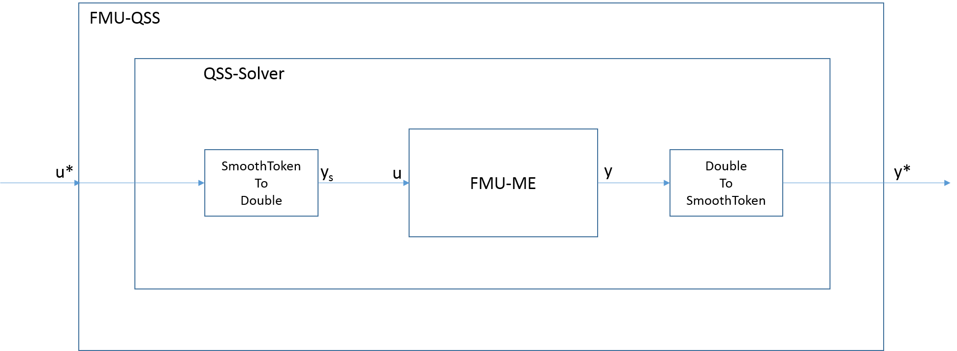
Fig. 5.5 : Conversion of input signal between FMU-QSS and FMU-ME.

To avoid frequent changes in the input signal, each input signal will have a quantum defined. The quantum \(\delta q\) will be computed at runtime as

\[\delta q = \max(\epsilon_{rel} \, |u^-|, \epsilon_{abs}),\]

where \(\epsilon_{rel}\) is the relative tolerance, \(u^-\) is the last value seen at the input of FMU-ME, and \(\epsilon_{abs} \triangleq \epsilon_{rel} \, |u_{nom}|\), where \(u_{nom}\) is the nominal value of the variable \(u\). During initialization, we set \(u^- = u_0\). The input signal will be updated only if it has changed by more than a quantum,

\[|y_s(t) - u^-| \ge \delta q.\]

To parametrize the smooth token, we propose to extend the FMI for model exchange specification to include fmi2SetRealInputDerivatives and fmi2GetRealOutputDerivatives. These two functions exist in the FMI for co-simulation API.

Note

• If a tool can not provide the derivative of an output variable with respect to time, fmi2GetRealOutputDerivatives then a master algorithm could approximate the output derivative as follows:

  • If there was no event, then the time derivatives from below and above are equal, and hence past and current output values can be used, e.g.,

    \[dy/dt \approx \frac{y(t_k)-y(t_{k-1})}{t_k - t_{k-1}}.\]

  • If there was an event, then the derivative from above need to be approximated. This could be done by assuming first \(dy/dt =0\) and then building up derivative information in the next step, or by evaluating the FMU for \(t=t_k+\epsilon\), where \(\epsilon\) is a small number, and then computing

    \[dy/dt \approx \frac{y(t_k+\epsilon)-y(t_{k})}{\epsilon}.\]

• For FMU-ME, if there is a direct feedthrough, e.g., \(y=f(u)\), then \(dy/dt\) cannot be computed, because by the chain rule,

  \[\frac{df(u)}{dt} = \frac{df(u)}{du} \, \frac{du}{dt}\]

  but \(du/dt\) is not available in the FMU.

5.4.1.7. Summary of Proposed Changes

To be updated

Here is a list with a summary of proposed changes

• fmi2SetReal can be called during the continuous, and event time mode for continuous-time states.

• The <Derivatives> element of the model description file will be extended to include higher order derivatives information.

• A new <EventIndicators> element wil be added to the model description file. This element will expose event indicators with their dependencies and time derivatives.

• If a model has an event indicator, and the event indicator has a direct feedthrough on an input variable, then OPTIMICA will exclude the derivatives of that event indicator from the model description file.

• A new dependency attribute eventIndicatorsDependencies will be added to state derivatives listed in the <Derivatives> element to include event indicators on which the state derivatives depend on.

• OPTIMICA will convert time event into state events, generate event indicators for those state events, and add those event indicators to the eventIndicatorsDependencies of state derivatives which depend on them.

• A new function fmi2SetRealInputDerivatives will be included to parametrize smooth token.

• A new function fmi2GetRealOutputDerivatives will be included to parametrize smooth token.

• All proposed XML changes will be initially implemented in the VendorAnnotation element of the model description file until they got approved and included in the FMI standard.

Note

• We need to determine when to efficiently call fmi2CompletedIntegratorStep() to signalize that an integrator step is complete.

• We need to determine how an FMU deals with state selection, detect it, and reject it on the QSS side.

5.4.1.8. Open Topics

This section includes a list of measures which could further improve the efficiency of QSS. Some of the measures should be implemented and benchmarked to ensure their necessity for QSS.

5.4.1.8.1. Atomic API

A fundamental property of QSS is that variables are advanced at different time rates. To make this practically efficient with FMUs, an API for individual values and derivatives is essential.

5.4.1.8.2. XML/API

All variables with non-constant values probably need to be exposed via the xml with all their interdependencies. The practicality and benefit of trying to hide some variables such as algebraic variables by short-circuiting their dependencies in the xml (or doing this short-circuiting on the QSS side) should be considered for efficiency reasons.

5.4.1.8.3. Higher Derivatives

Numerical differentiation significantly complicates and slows the QSS code: automatic differentiation provided by the FMU will be a major improvement and allows practical development of 3rd order QSS solvers.

5.4.1.8.4. Input Variables

• Input functions with discontinuities up to the QSS order need to be exposed to QSS and provide next event time access to the master algorithm.

• Input functions need to be true (non-path-dependent) functions for QSS use or at least provide a way to evaluate without “memory” to allow numeric differentiation and event trigger stepping.

5.4.1.8.5. Annotations

Some per-variable annotations that will allow for more efficient solutions by overriding global settings (which are also needed as annotations) include:

• Various time steps: dt_min, dt_max, dt_inf, …

• Various flags: QSS method/order (or traditional ODE method for mixed solutions), inflection point requantization, …

• Extra variability flags: constant, linear, quadratic, cubic, variable, …

5.4.1.8.6. Conditional Expressions and Event Indicators

• How to reliably get the FMU to detect an event at the time QSS predicts one?

  QSS predicts zero-crossing event times that, even with Newton refinement, may be slightly off. To get the FMU to “detect” these events with its “after the fact” event indicators the QSS currently bumps the time forward by some epsilon past the predicted event time in the hopes that the FMU will detect it. Even if made smarter about how big a step to take this will never be robust. Missing events can invalidate simulations. If there is no good and efficient FMU API solution we may need to add the capability for the QSS to handle “after the fact” detected events but with the potential for large QSS time steps and without rollback capability this would give degraded results at best.

• How much conditional structure should we expose to QSS?

  Without full conditional structure information the QSS must fire events that aren’t relevant in the model/FMU. This will be inefficient for models with many/complex conditionals. These non-event events also alter the QSS trajectories so, for example, adding a conditional clause that never actually fires will change the solution somewhat, which is non-ideal.

• QSS needs a mechanism similar to zero crossing functions to deal with Modelica’s event generating functions (such as div(x,y) See http://book.xogeny.com/behavior/discrete/events/#event-generating-functions) to avoid missing solution discontinuities.

• Discrete and non-smooth internal variables need to be converted to input variables or exposed (with dependencies) to QSS.

• QSS need dependency information for algebraic and boolean/discrete variables either explicitly or short-circuited through the exposed variables for those the QSS won’t track.

• The xml needs to expose the structure of each conditional block: if or when, sequence order of if/when/else conditionals, and all the (continuous and discrete/boolean) variables appearing in each conditional.

• Non-input boolean/discrete/integer variables should ideally be altered only by event indicator handlers or time events that are exposed by the FMU (during loop or by direct query?). Are there other ways that such variables can change that are only detectable after the fact? If so, this leaves the QSS with the bad choices of late detection (due to large time steps) or forcing regular time step value checks on them.

• QSS needs the dependencies of conditional expressions on variables appearing in them.

• QSS needs the dependencies of variables altered when each conditional fires on the conditional expression variables.

• It is not robust for the QSS to try and guess a time point where the FMU will reliably detect a zero crossing so we need an API to tell the FMU that a zero crossing occurred at a given time (and maybe with crossing direction information).

• If the xml can expose the zero crossing directions of interest that will allow for more efficiency.

5.5. Integration with OpenStudio

The integration with OpenStudio will be done through an html5 widget. The development of this link is documented at https://github.com/lbl-srg/linkage.js