6. Numerical Methods of the Master Algorithm

This section describes the numerical methods that are used by the master algorithm.

First, we note that conventional continuous time integration algorithms have the following fundamental properties in common [CK06]: Given a time \(t_{k+1}\), a polynomial approximation is performed to determine the values of all state variables at that time instant. If an error estimate is too large, the computation is repeated with a shorter time step. If an event happened, an iteration takes place across all states to determine when the event occurred. At the event, the approximations of the higher-order derivatives, which are the basis for multi-step methods, become invalid. Hence multi-step methods need to be restarted with a low-order method. This is very expensive as it involves a global event iteration followed by an integrator reset to a low order method. As event iteration is computationally expensive, and as our models will have a large number of state events, we will use a different integration method based on the Quantized State System (QSS) representation.

6.1. Time Integration

QSS methods follow entirely different approach: Let \(t_k\) be the current time. We ask each state individually at what time \(t_{k+1}\) it will deviate more than a quantum \(\Delta q> 0\) from its current value. This is a fundamentally different approach as the state space is discretized, rather than time, and all communication occurs through discrete events. Furthermore, when a state variable changes to a new quantization level, the change need only be communicated to other components whose derivatives depend on that state, hence communication is local. We thus selected for the SOEP QSS as our integration methods.

QSS algorithms are new methods that are fundamentally different from standard DAE or ODE solvers. The volume of literature about QSS methods is today where ODE solvers were about 30 years ago. QSS methods have interesting properties as they naturally lead to asynchronous integration with minimal communication among state variables. They also handle state events explicitly without requiring an iteration in time to solve zero-crossing functions.

The first order QSS method, QSS1, first appeared in the literature in 1998 [ZL98]. QSS1 methods have been extended to second and third order methods (QSS2, QSS3). On non-stiff problems, QSS3 has been shown to be significantly faster than QSS, and in some cases were faster than DASSL in Dymola [FBCK11]. To address performance issues observed in QSS, the class of Linear Implicit QSS methods (LIQSS) have been developed for stiff systems [Kof06] [MBKC13]. For stiff systems, the 3rd order implementation of LIQSS seems to perform best as shown in Fig. 6.1, which is from [MBKC13].

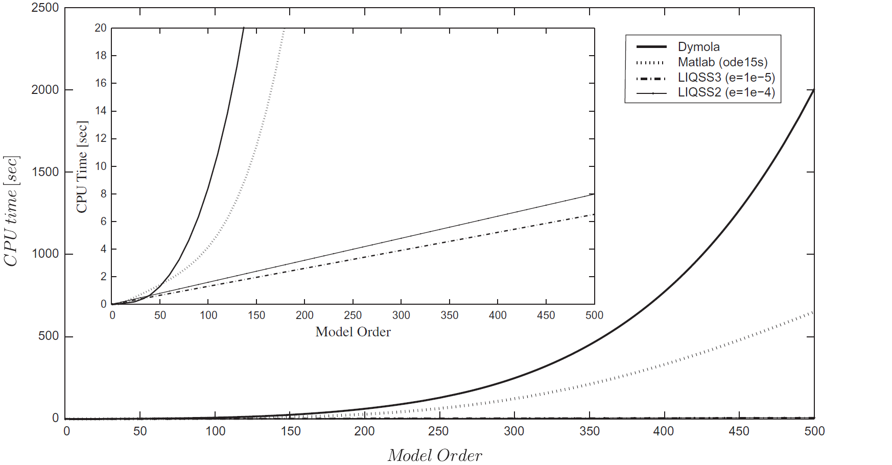
Fig. 6.1 : LIQSS method have linear growth of computing time, whereas ode15 (MATLAB) and esdirk23a (Dymola) have cubic growth.

Over the past years, different classes of QSS algorithms have been implemented. The next section describes how these algorithms differ from one another. We also give insights into which algorithms appear to be suitable for the SOEP.

6.1.1. QSS1

We will first discuss QSS1 and then show how it has been extended to higher order and implicit QSS methods. Consider the following ODE

(6.1)\[\dot x(t) = f (x(t), u(t)),\]

with \(t \in [t_0, \, t_f]\), and initial conditions \(x(t_0) = x_0\), where \(x(t) \in \Re^n\) is the state vector and \(u(t) \in \Re^m\) is the input vector. For simplicity, suppose \(u(\cdot)\) is piece-wise constant. The QSS1 method solves analytically an approximate ODE, which is called QSS, of the form

(6.2)\[\dot x(t) = f (q(t), u(t)),\]

where \(q(t)\) is a vector of quantized values of the state \(x(t)\). Each component \(q_i(t)\) of \(q(t)\) follows a piecewise constant trajectory, related with the corresponding component \(x_i(t)\) by a hysteretic quantization function. The hysteretic quantization function is defined as follows: For some \(K \in \mathbb N_+\), let \(j \in \{0, \ldots, K-1\}\) denote the counter for the time intervals. Then, for \(t_j \le t < t_{j+1}\), the hysteretic quantization function is defined as

(6.3)\[\begin{split} q_i (t) = \begin{cases} x_i(t), & \text{if } |x_i (t)-q_i(t^{-})| = \Delta q_i, \\ q_i(t_j), & \text{otherwise}, \end{cases}\end{split}\]

with initial condition \(q_i(t_0) = x_i(t_0)\), where the sequence \(\{t_{j}\}_{j=0}^{K-1}\) is constructed as

\[t_{j+1} = \min \{t \in \Re \, | \, t > t_j, \, |x_i(t_j) - x_i(t)| = \Delta q_i \}.\]

Thus, the component \(q_i(t)\) changes its state when it differs from \(x_i(t)\) by \(\pm\Delta q_i\). Fig. 6.2 shows an example of a quantization function for QSS1.

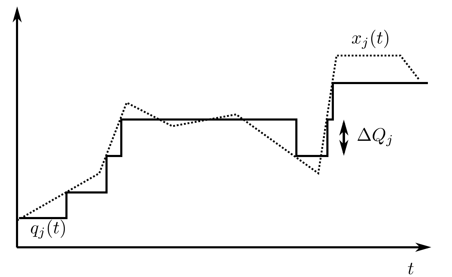
Fig. 6.2 : Example of quantization function for QSS1.

Example

For illustration, consider the following differential equation where on the left, we have the original form, and on the right, we have its QSS form. Here, we took the simplest quantization function, e.g, the ceiling function \(q(x)=\lceil{x}\rceil = \arg \min_{z \in \mathbb Z} \{ x \le z \}\), but in practice, finer spacing with hysteresis is used for higher accuracy and to avoid chattering. Consider

\[\begin{split}\begin{aligned}[c] \dot x_1(t) & = - x_1(t) \\ \dot x_2(t) & = - 2 \, x_1(t) \\ \dot x_3(t) & = - 2 \, \left( 2 \, x_2(t) + x_3(t) \right) \\ x(0) & = (10, 10, 10) \end{aligned} \qquad\xrightarrow{\text{QSS1}}\qquad \begin{aligned}[c] \dot \chi_1(t) & = - \lceil{\chi_1(t)}\rceil \\ \dot \chi_2(t) & = - 2 \, \lceil{\chi_1(t)}\rceil \\ \dot \chi_3(t) & = - 2 \, \left( 2 \, \lceil{\chi_2(t)}\rceil + \lceil{\chi_3(t)}\rceil \right) \\ \chi(0) & = (10, 10, 10) \end{aligned}\end{split}\]

Fig. 6.3 shows the time series of the solution of the differential equation computed by QSS1.

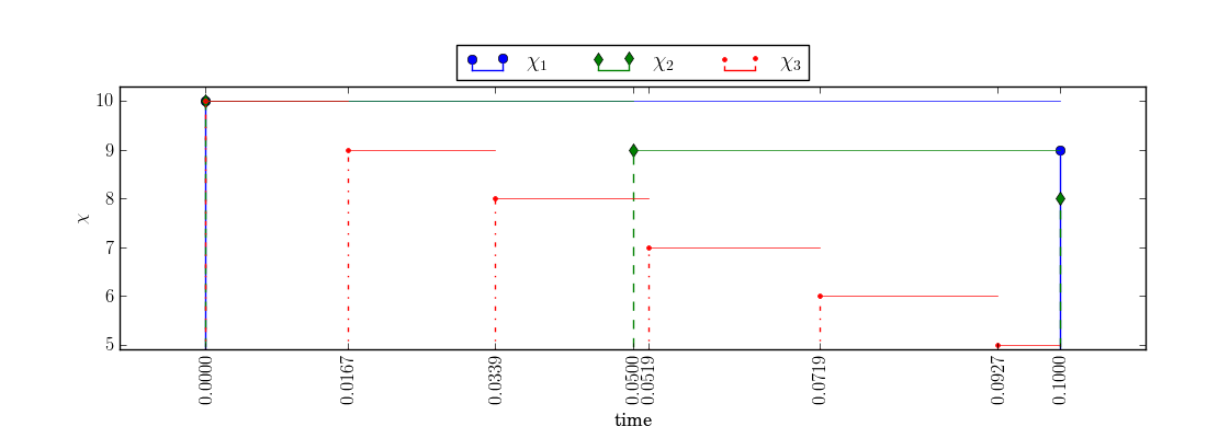
Fig. 6.3 : Time series computed by QSS1 for \(t \in [0, 0.1]\).

The computation is as follows: In QSS, each state can be integrated asynchronously until its right-hand side changes. Therefore, we can compute directly the first transitions as \(\chi_1(0.1) = 9\), \(\chi_2(0.05) = 9\), \(\chi_3(0.01667) = 9\). We can keep integrating \(\chi_3(\cdot)\) until its input \(\chi_2(\cdot)\) changes, which will be at \(t=0.05\). Thus, we compute \(\chi_3(0.0339) = 8\). The next transition of \(\chi_3(\cdot)\) would be at \(t=0.0518\). But \(\chi_2(\cdot)\) transitions from \(10\) to \(9\) at \(t=0.05\) so we can not integrate beyond that. Hence, we compute the next potential transition of \(\chi_3(\cdot)\) (from \(8\) to \(7\)) as \(t = 0.05190 = \arg \min \{\Delta \in \Re_0^+ \, | 7 = 8 + \int_{0.0339}^{0.05} (-2 \, (2 \cdot 10 + 8) \, ds + \int_{0.05}^{\Delta} (-2 \, (2 \cdot 9+8)) \, ds\}\). Hence, \(\chi_3(\cdot)\) will transition next at \(t=0.05190\) provided that its input does not change within this time. The input won’t change because the next transition of \(\chi_2(\cdot)\) will be \(\chi_2(0.1) = 8\). Therefore, we integrate \(\chi_3(\cdot)\) until \(t=0.1\), at which time \(\chi_1(\cdot)\) and \(\chi_2(\cdot)\) transition.

6.1.2. QSS2

We will now describe the second order QSS2 method. This method replaces the simple hysteretic quantization function of QSS1 (6.3) with a first order-quantizer. This leads, for \(t_j \leq t < t_{j+1}\), to

\[\begin{split}q_i(t) = \begin{cases} x_i(t), & \text{if } |x_i(t)-q_i(t^{-})| = \Delta q_i, \\ q_i(t_j) + m_{ij} (t-t_j), & \text{otherwise}, \end{cases}\end{split}\]

with initial condition \(q_i(t_0) = x_i(t_0)\), where the sequence \(\{t_{j}\}_{j=0}^{K-1}\) is constructed as

\[t_{j+1} = \min \{t \in \Re \, | \, t > t_j, \, |x_i(t_j) + m_{ij} (t-t_j) - x_i(t)| = \Delta q_i \},\]

with the slope \(m_{ij}\) defined as \(m_{i0}=0\) and \(m_{ij}= \dot x_i(t_j^-)\) for \(j \in \{1, \ldots, K-1\}\).

Note

For \(m_{ij}\), the limit from below \(\dot x_i(t_j^-)\) is used.

The figure below shows an example of a quantization function for QSS2.

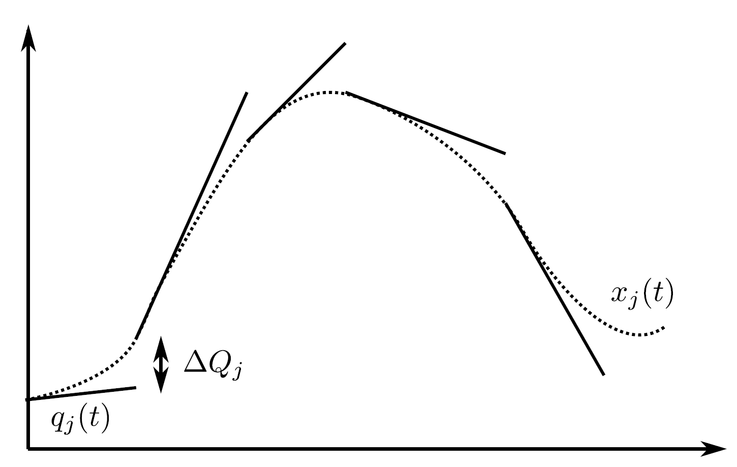
Fig. 6.4 : Example of quantization function for QSS2.

6.1.3. QSS3

In QSS3, the trajectories of \(x_i(t)\) and \(q_i(t)\) are related by a second order quantization function. This leads, for \(t_j \leq t < t_{j+1}\), to

\[\begin{split}q_i(t) = \begin{cases} x_i(t), & \text{if } |x_i(t)-q_i(t^{-})| = \Delta q_i, \\ q_i(t_j) + m_{ij} (t-t_j) + p_{ij} (t-t_j)^2, & \text{otherwise}, \end{cases}\end{split}\]

with initial condition \(q_i(t_0) = x_i(t_0)\), where the sequence \(\{t_{j}\}_{j=0}^{K-1}\) is constructed as

\[t_{j+1} = \min \{t \in \Re \, | \, t > t_j, \, |x_i(t_j) + m_{ij} (t-t_j) + p_{ij} (t-t_j)^2 - x_i(t)| = \Delta q_i \},\]

with the slopes defined as \(m_{i0}=0\) and \(m_{ij}= \dot x_i(t_j^-)\), for \(j \in \{1, \ldots, K-1\}\), for the first order term, and \(p_{i0}=0\) and \(p_{ij}= \dot m_{ij}\) for the second order term.

6.1.4. Discussion of QSS

QSS1, QSS2, and QSS3 are efficient for the simulation of non-stiff ODEs.

The number of integration steps of QSS1 is inversely proportional to the quantum. For QSS2, it is inversely proportional to the square root of the quantum. For QSS3, it is inversely proportional to the cubic root of the quantum. See [Kof06] for a derivation.

However, they have been shown to exhibit oscillatory behavior, with high computing time, if applied to stiff ODEs [MBKC13]. In [MBKC13], they were extended to LIQSS methods. As building simulation models can be stiff, we will now present these methods.

6.1.5. LIQSS

We will now focus our discussion on LIQSS methods, which seem to be the most applicable classes of QSS methods for building simulation. We will start our discussion with the first order LIQSS (LIQSS1) and expand the discussion to higher order LIQSS methods. The basic idea of LIQSS1 is to select the value of \(q_i(t)\) so that \(x_i(t)\) approaches \(q_i(t)\). This implies that \((q_i(t)-x_i(t)) \, \dot {x}_i(t) \geq 0\) for \(t_j \leq t < t_{j+1}\). Given the ODE defined in (6.1), LIQSS1 approximates it by (6.2), where each \(q_i(t)\) is defined in [MK07] as

\[\begin{split}q_i(t) = \begin{cases} \underline{q}_i(t), & \text{if } f_{i}(q(t), u(t)) \,(\underline{q}_i(t) - x_{i}(t)) \geq 0, \\ \bar{q}_i(t), & \text{if } f_{i}(q(t), u(t)) \,(\bar{q}_i(t) - x_{i}(t)) \geq 0 \land f_{i}(q(t), u(t)) \,(\underline{q}_i(t) - x_{i}(t)) < 0, \\ \tilde{q}_i(t), & \text{otherwise}, \end{cases}\end{split}\]

with

\[\begin{split}\underline{q}_i(t) & = \begin{cases} \underline{q}_i(t^-) - \Delta q_i, & \text{if } x_i(t) - \underline{q}_i(t^-) \le 0, \\ \underline{q}_i(t^-) + \Delta q_i, & \text{if } x_i(t) - \underline{q}_i(t^-) \ge 2 \, \Delta q_i, \\ \underline{q}_i(t^-), & \text{otherwise,}\\ \end{cases}\\ \bar q_i(t) & = \underline{q}_i(t) + 2 \, \Delta q_i, \\ \tilde q_i(t) & = \begin{cases} \bar q_i(t) - \frac{1}{A_{i,i}} f_i(\bar {q}^i(t), u(t)), & \text{if } A_{i,i} \not = 0,\\ q_i(t^-), & \text{otherwise,}\\ \end{cases}\end{split}\]

where \(A_{i,i}\) is an estimate of the \(i\)-th diagonal element of the Jacobian. For its computation, and for how to compute \(\bar {q}^i(t)\), we refer to [MK07].

Higher order LIQSS methods (e.g. LIQSS2, LIQSS3) combine the ideas of higher order QSS methods and LIQSS. Reference [MBKC13] gives a detailed formal definition of such methods. Rather than using the first order condition, the \(N\)-th order method LIQSSN uses \((q_i(t)-x_i(t)) \, x_i^{(N)}(t) \geq 0\), where \(x_i^{(N)}: \Re \rightarrow \Re\) is the \(N\)-th order derivative of \(x_i( \cdot)\) with respect to time.

6.1.6. Discussion of LIQSS

LIQSS methods are efficient for stiff systems where the stiffness is reflected in large diagonal elements of the Jacobian matrix. This is due to the fact that LIQSS solvers avoid fast oscillations by using information derived from the diagonal of the Jacobian matrix. When stiffness is not due to the diagonal elements of the Jacobian matrix, then LIQSS can also exhibit oscillatory behavior [MBKC13].

6.2. Algebraic Loops

This section discusses algebraic loops which can occur when modeling systems with feedback. In block diagrams, algebraic loops occur when the input of a block with direct feedthrough is connected to the output of the same block, either directly, or by a feedback path through other blocks which all have direct feedthrough.

Algebraic loops are generally introduced when the dynamics of a component is approximated by its steady-state solution. For the SOEP, subsystems that form algebraic loops include:

1. The infrared radiation network within a thermal zone. This is not a problem as this system of equations is likely to be contained inside an FMU. Hence, an FMU can output the solution to this system of algebraic equations.

2. Flow networks such as a water loop. Algebraic loops can be formed for the energy balance, mass balance and the pressure network. For the energy and mass balance, these loops can be eliminated by adding a transport delay that approximates the travel time of the fluid inside the pipe. For the pressure network, an approximation through the speed of sound is not suited as this would lead to very fast transients. Therefore, we will need a means to solve systems of algebraic equations that are formed by coupling multiple FMUs with direct feedthrough.

Such algebraic loops are generally solved using Newton-Raphson type algorithms. In the next section, we describe the requirements of these methods.

6.2.1. Software Requirements for Efficient Implementation of Newton-Raphson Method for Algebraic Loops

The following requirements are needed by SOEP FMUs to ensure that they can be efficiently solved using the Newton-Raphson method:

1. FMUs need to provide information about their input dependencies. This information is stored in the model description file of the FMU as output dependency under the element <ModelStructure>. In FMI 2.0, this data is specified as optional. For SOEP, we require the output dependency to be declared as the master requires it to determine the existence and location of algebraic loops. Note that a connection between input and output only causes an algebraic loop if the output depends algebraically on the input. Integrators, however, break algebraic loops.

2. FMUs need to provide derivatives of their outputs with respect to their inputs. This information is needed by the Newton-Raphson method. The Newton-Raphson method finds the root of the residual function \(f(x) = y-x\). The root of this function is calculated iteratively as \(x_{k+1}=x_k -{y_k}/{f'(x_k)}\) with \(f'(x) = {df(x)}/{dx}\). If the derivative with respect to the input cannot be provided, then the derivative would need to be approximated numerically. This is computationally costly and less robust than providing derivative functions.