Unscented Kalman Filter and Smoother¶

This module contains a class that provides functionalities for solving state estimation problems with the Unscented Kalman Filter (UKF) and the Unscented Kalman Smoother. The algorithm works with models that are compliant with the FMI standard [3]. This documentation provides information about the method used by the class, we suggest the interested readers to refer to [Julier1996], [Julier2002], [Sarkka2007], and [Sarkka2008] for more information on UKF and the smoother. Also, details on the implementation of EstimationPy were presented in [Bonvini2014].

State Estimation

Kalman Filter (KF) [Haykin2001] are often used to estimate state variables. However, as they are only applicable for linear systems, they are not suited for our applications. For systems that are described by nonlinear differential equations, the state estimation problem can be solved using an Extended Kalman Filter (EKF) [Haykin2001]. The EKF linearizes around the current state estimate the original nonlinear model. However, in some cases, this linearization introduces large errors in the estimated second order statistics of the estimated state vector probability distribution [WanMerwe2000]. Another approach is to simulate sample paths that generate random points in the neighborhood of the old posterior probability, for example by using Monte Carlo sampling, and adopting particle filters for the state estimation [Doucet2002]. These techniques are robust with respect to model nonlinearities, but they are computationally expensive. The UKF faces the problem representing the state as a Gaussian random variable, the distribution of which is modeled non parametrically using a set of points known as sigma points [Julier1996]. Using the sigma points, i.e., by propagating a suitable number of state realizations through the state and output equations, the mean and the covariance of the state can be captured. The favorable properties of the UKF makes its computational cost far lower than the Monte Carlo approaches, since a limited and deterministic number of samples are required. Furthermore, the UKF requirements fit perfectly with the infrastructure provided by PyFMI since it provides an interface to the FMU model that allows to set state variables, parameter and running simulations.

The Unscented Kalman Filter

The Unscented Kalman Filter is a model based-techniques that recursively estimates the states (and with some modifications also parameters) of a nonlinear, dynamic, discrete-time system. This system may for example represent a building, an HVAC plant or a chiller. The state and output equations are

(1)\[\begin{split}\begin{align} \mathbf{x}(t_{k+1}) &= f(\mathbf{x}(t_k), \mathbf{u}(t_k), \Theta(t), t) + \mathbf{q}(t_k), \\ \mathbf{y}(t_k) &= H(\mathbf{x}(t_k),\mathbf{u}(t_k), \Theta(t), t) + \mathbf{r}(t_k), \end{align}\end{split}\]

with initial conditions \(\mathbf{x}(t_0) = \mathbf x_0\), where \(f \colon \Re^n \times \Re^m \times \Re^p \times \Re \to \Re^n\) is nonlinear, \(\mathbf{x}(\cdot) \in \mathbb{R}^n\) is the state vector, \(\mathbf{u}(\cdot) \in \mathbb{R}^m\) is the input vector, \(\Theta(\cdot) \in \mathbb{R}^p\) is the parameter vector, \(\mathbf{q}(\cdot) \in \mathbb{R}^n\) represents the process noise (i.e. unmodeled dynamics and other uncertainties), \(\mathbf{y}(\cdot) \in \mathbb{R}^o\) is the output vector, \(H \colon \Re^n \times \Re^m \times \Re^p \times \Re \to \Re^o\) is the output measurement function and \(\mathbf{r}(\cdot) \in \mathbb{R}^o\) is the measurement noise.

The UKF is based on the typical prediction-correction style methods

PREDICTION STEP: predict the state and output at time step \(t_{k+1}\) by using the parameters and states at \(t_{k}\).

CORRECTION STEP: given the measurements at time \(t_{k+1}\), update the posterior probability, or uncertainty, of the states prediction using Bayes’ rule.

The original formulation of the UKF imposes some restrictions on the model because the system needs to be described by a system of initial-value, explicit difference equations (1). A second drawback is that the explicit discrete time system cannot be used to simulate stiff systems efficiently. The UKF should be translated in a form that is able to deal with continuous time models, possibly including events.

Although physical systems are often described using continuous time models, sensors routinely report time-sampled values of the measured quantity (e.g. temperatures, pressures, positions, velocities, etc.). These sampled signals represent the available information about the system operation and they are used by the UKF to compute an estimation for the state variables.

A more natural formulation of the problem is represented by the following continuous-discrete time model

(2)\[\begin{split}\begin{align} \frac{d \ \mathbf{x}(t)}{dt} &= F(\mathbf{x}(t), \mathbf{u}(t), \Theta(t), t), \\ \mathbf{x}(t_0) &= \mathbf{x}_0, \\ \mathbf{y}(t_k) &= H(\mathbf{x}(t_k),\mathbf{u}(t_k), \Theta(t), t_k) + \mathbf{r}(t_k), \end{align}\end{split}\]

where the model is defined in the continuous time domain, but the outputs are considered as discrete time signals sampled at discrete time instants \(t_k\). The original problem described in equation can be easily derived as

(3)\[\begin{split}\mathbf{x}(t_{k+1}) &=& f(\mathbf{x}(t_k), \mathbf{u}(t_k), \Theta(t_k), t_k) \nonumber \\ &=& \mathbf{x}(t_k) + \int_{t_k}^{t_{k+1}} F(\mathbf{x}(t), \mathbf{u}(t), \Theta(t), t)\, dt\end{split}\]

EstimationPy implementation uses this continuous-discrete time formulation and the numerical integration is done using PyFMI that works with a model embedded as an FMU. Despite not shown, in (2) and (3) the model may contain events that are handled by the numerical solver provided with the PyFMI package.

The UKF is based on the the Unscented Transformation [Julier1996] (UT), which uses a fixed (and typically low) number of deterministically chosen sigma-points [4] to express the mean and covariance of the original distribution of the state variables \(\mathbf{x}(\cdot)\), exactly, under the assumption that the uncertainties and noise are Gaussian [Julier1996]. These sigma-points are then propagated simulating the nonlinear model (2) and the mean and covariance of the state variables are estimated from them. This is significantly different from Monte Carlo approaches because the UKF chooses the points in a deterministic way. One of the most important properties of this approach is that if the prior estimation is distributed as a Gaussian random variable, the sigma points are the minimum amount of information needed to compute the exact mean and covariance of the posterior after the propagation through the nonlinear state function [WanMerwe2000].

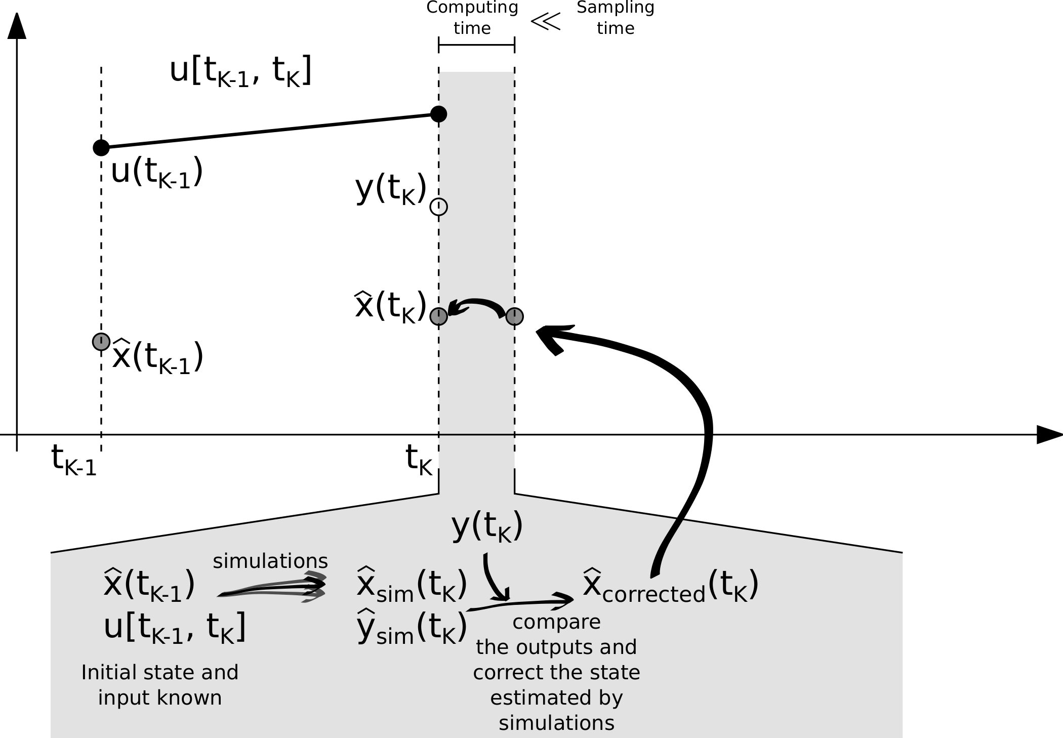
The above Figure illustrates the filtering process which we will now explain. At time \(t_k\), a measurement of the outputs \(\mathbf{y}(t_k)\), the inputs and the previous estimation of the state are available. Simulations are performed starting from the prior knowledge of the state \(\hat{\mathbf{x}}(t_{k-1})\), using the input \(\mathbf{u}(t_{k-1})\). Once the results of the simulations \(\hat{x}_{sim}(t_k)\) and \(\hat{y}_{sim}(t_k)\) are available, they are compared against the available measurements in order to correct the state estimation. The corrected value (i.e. filtered) becomes the actual estimation. Because of its speed, the estimation can provide near-real-time updates, since the time spent for simulating the system and correcting the estimation is typically shorter than the sampling time step, in particular for building or HVAC applications, where computations take fractions of second and sampling intervals are seconds or minutes.

Smoothing to Improve UKF Estimation

In this subsection, we discuss an additional refinement procedure to the UKF. The distribution \(P(\mathbf{x}(t_k) \vert \mathbf{y}(t_1), \dots , \mathbf{y}(t_k))\) is the probability to observe the state vector \(\mathbf{x}(t_k)\) at time \(t_k\) given all the measurements collected. By using more data \(P(\mathbf{x}(t_k) \vert \mathbf{y}(t_1), \dots , \mathbf{y}(t_k), \dots \mathbf{y}(t_{k+N}))\), the posterior distribution can be improved through recursive smoothing. Hence, the basic idea behind the recursive smoothing process is to incorporate more measurements before providing an estimation of the state.

The above Figure represents the smoothing process. While the filter works forwardly on the data available, and recursively provides a state estimation, a smoothing procedure back-propagates the information obtained during the filtering process, after some amount of data becomes available, in order to improved the estimation previously provided [Sarkka2008].

The smoothing process can be viewed as a delayed, but improved, estimation of the state variables. The longer the acceptable delay, the bigger the improvement since more information can be used. For example if, at a given time, a sensor provides a wrong measurement, the filter may not be aware of this and it may provide an estimation that does not correspond to the real value (although the uncertainty bounds will still be correct). The smoother observes the trend of the estimation will reduce this impact of the erroneous data, thus providing an estimation that is less sensitive to measurement errors.

Parameter Estimation

The importance of the state estimation has been stressed, and we described the UKF and Smoother as solutions to this problem. While state estimation is particularly important for controls, parameter estimation is important for model calibration and fault detection and diagnostics. Consider, for example an heat exchanger. Suppose it is characterized by one heat exchange coefficient that influences the heat transfer rate between the two fluids. During the design of the heat exchanger it is possible to compute an approximation of it. However, it is not possible to know its value exactly. After the heat exchanger is created, identifying the value of it is important to verify if the design requirements have been met. Another example is real-time monitoring in which it is continuously monitored during the operation in order to continuously check if it has been reduced by fouling and the heat exchanger need to be serviced.

Continuous parameter estimation is possible by extending the capabilities of the UKF and Smoother to estimate not just the state variable, but also the parameters of the system. The approach is to include the parameter in an augmented state \(\mathbf{x}^A(\cdot)\), defined as

\[\mathbf{x}^A(\cdot) = \left [ \mathbf{x}(\cdot) \ \ \ \mathbf{x}^P(\cdot) \right ]^T,\]

where \(\mathbf{x}^P(\cdot) \subseteq \Theta(\cdot)\) is a vector containing a subset of the full parameter vector \(\Theta(\cdot)\) to be estimated. The new components of the state variables need a function that describe their dynamics. Since in the normal operation, these values are constant, the associated dynamic is

\[\frac{d \ \mathbf{x}^P(t) }{dt} = \mathbf{0},\]

where \(\mathbf{0}\) is a null vector. These null dynamics have to be added (2). The result is a new continuous-discrete time system

\[\begin{split}\begin{align} \frac{d \ \mathbf{x}^A(t)}{dt} &= F_A(\mathbf{x}^A(t), \mathbf{u}(t), \Theta(t), t) \\ \mathbf{y}(t_k) &= H(\mathbf{x}^A(t_k),\mathbf{u}(t_k), \Theta(t_k), t_k) + \mathbf{r}(t_k), \end{align}\end{split}\]

with

\[\begin{split}F_A(\mathbf{x}^A(t), \mathbf{u}(t), \Theta(t), t) = \begin{bmatrix} F(\mathbf{x}(t), \mathbf{u}(t), \Theta(t), t) \\ \mathbf{0} \end{bmatrix}\end{split}\]

Note that augmenting the state variables leads to a nonlinear state equation even if \(F(\cdot, \cdot, \cdot, \cdot)\) is a linear function. Therefore, for parameter estimation, a nonlinear filtering and smoothing technique is required.

Notation¶

The superscript \(^{(i)}\) indicates that the quantity is related to the i-th sigma point, \(w_m^{(i)}\) and \(w_c^{(i)}\) are the weights associated to the \(i-th\) sigma point, \(N\) is the dimension of the state vector \(\mathbf{x}(\cdot)\), and \([\cdot]_i\) is an operator that if applied to a matrix \(A\) returns its \(i-th\) column. Vectors are indicated with bold characters.

class estimationpy.ukf.ukf_fmu.UkfFmu(model, n_proc=3)¶

This class represents an Unscented Kalman Filter (UKF) that can be used for the state and parameter estimation of nonlinear dynamic systems represented by FMU models.

This class uses an object ot type estimationpy.fmu_utils.model.Model to represent the system. The model once instantiated and configured, already contains the data series associated to the measured inputs and outputs, the list of states and parameters to estimates, covariances, and constraints for the estimated variables. See estimationpy.fmu_utils.model for more information.

The class internally uses an estimationpy.fmu_utils.fmu_pool.FmuPool to run simulations in parallel over multiple processors. Please have a look to estimationpy.fmu_utils.fmu_pool for more information.

__init__(model, n_proc=3)¶

Constructor of the class that initializes an object that can be used to solve state and parameter estimation problems by using the UKF and smoothing algorithms. The constructor requires a model representing the systems which states and/or parameters will be estimated.

The method performs the following steps

creates a reference to the models and instantiales an object of type estimationpy.fmu_utils.fmu_pool.FmuPool for running simulations in parallel,
compute the number of sigma points to be used,
define the parameters of the filter,
compute the weights associated to each sigma point,
initialize the constraints on the observed state variables and estimated parameters,

Parameters:

model (estimationpy.fmu_utils.model.Model) – the model which states and/or parameters have to be estimated.
n_proc (int) – a positive integer that defines the number of processes that are created when the simulations are run. Make sure this value is equal to 1 if the filtering or smoothing are executed as part of a Celery task. By default this value is equal to the number of available processors minus one.

Raises:

ValueError – The method raises an exception if the model associated to the filter does not have state or parameters to be estimated.
Exception – The method raises an exception if there are not measured outputs, the number of states to estimate is higher than the total number of states, of the number of parameters to estimate is invalid.

__str__()¶

This method returns a string representation of the object with a brief description containing

name of the model,
total number of states,
total number of observed states,
total number of parameters to estimate, and
number of measured outputs used to perform the estimation.

Returns:	string representation of the object
Return type:	string

average_proj(x)¶

This function averages the projection of the sigma points. The function can be used to compute the average of both the state vector or the measured outputs. The weigths vetcor used is \(\mathbf{w}_m\).

Parameters:	x (np.ndarray) – the vector to average \(\mathbf{x}\)
Returns:	the average of the vector computed as \(\mathbf{w}_m^T \mathbf{x}\)
Return type:	numpy.ndarray

chol_update(L, X, W)¶

This method computes the Cholesky update of a matrix.

Parameters:	L (numpy.ndarray) – lower triangular matrix computed with QR factorization X (numpy.array) – vector used to compute the covariance matrix. It can either be a vector representing the deviation of the state from its average, or the deviation from an output from its average. W (numpy.array) – vector of weights
Returns:	the square root matrix computed using the Cholesky update
Return type:	numpy.ndarray

compute_C_x_x(x_new, x)¶

This method computes the state-state cross covariance matrix \(C_{xx}\) between the old state \(\mathbf{x}\) and the new state \(\mathbf{x}_{new}\).

\[C_{xx} = \sum_{i=0}^{2n+1} w_c^{(i)} \left ( \mathbf{x}_{new}^{(i)} - \boldsymbol{\mu}_{new} \right ) \left ( \mathbf{x}^{(i)} - \boldsymbol{\mu}) \right )^T\]

where \(\boldsymbol{\mu}\) and \(\boldsymbol{\mu}_{new}\) are the average of the vectors \(\mathbf{x}\) and \(\mathbf{x}_{new}\) over all the sigma points \(i\).

Notes: This is method is used by the smoothing process because during the smoothing the averages are not directly available and thus compute_cov_x_x() can’t be used.

Parameters:	x_new (numpy.array) – vector that contains the full state of the system (estimated, not estimated states, as well the estimated parameters), this vector can be seen as the propagated sigma points x (numpy.array) – vector containing initial states before the progatation
Returns:	state-state covariance matrix \(C_{xx}\)
Return type:	numpy.ndarray

compute_P(x, x_avg, Q)¶

This method computes the state covariance matrix \(P\) as

\[P = Q + \sum_{i=0}^{2n+1} w_c^{(i)} \left ( \mathbf{x}^{(i)} - \boldsymbol{\mu} \right ) \left ( \mathbf{x}^{(i)} - \boldsymbol{\mu} \right )^T\]

where \(\boldsymbol{\mu}\) is the average of the vector \(\mathbf{x}\) among the different sigma points. The method removes the not observed states from \(\mathbf{x}\) and computes the covariance matrix \(\mathbf{P}\).

Parameters:	x (numpy.array) – vector that conatins the estimated states of the system as well the estimated parameters. This vector can be seen as the propagated sigma points. x_avg (numpy.array) – vector that contains the average of the propagated sigma points Q (numpy.ndarray) – covariance matrix

compute_S(x_proj, x_ave, sqrt_Q, w=None)¶

This method computes the squared root covariance matrix using the QR decomposition combined with a Cholesky update. The matrix returned by this method is upper triangular.

Parameters:	x_proj (numpy.array) – projected full state vector x_avg (numpy.array) – average of the full state vector sqrt_Q (numpy.ndarray) – square root process covariance matrix w (numpy.array) – vector that contains the weights to use during the update. If not specified the method uses the weights automatically computed by the filter.
Returns:	the square root of the updated state covariance matrix. The matrix is upper triangular.
Return type:	nunmpy.ndarray

compute_S_y(y_proj, y_ave, sqrt_R)¶

This method computes the squared root covariance matrix using the QR decomposition combined with a Cholesky update.

Parameters:	y_proj (numpy.array) – projected measured output vector y_avg (numpy.array) – average of the measured output vector sqrt_R (numpy.ndarray) – square root process covariance matrix
Returns:	the square root of the updated output covariance matrix
Return type:	nunmpy.ndarray

compute_cov_x_x(x_new, x_new_avg, x, x_avg)¶

This method computes the state-state cross covariance matrix \(C_{xx}\). The different states are the state before and after the propagation.

\[C_{xx} = \sum_{i=0}^{2n+1} w_c^{(i)} \left ( \mathbf{x}_{new}^{(i)} - \boldsymbol{\mu}_{new} \right ) \left ( \mathbf{x}^{(i)} - \boldsymbol{\mu}) \right )^T\]

where \(\boldsymbol{\mu}\) and \(\boldsymbol{\mu}_{new}\) are the average of the vectors \(\mathbf{x}\) and \(\mathbf{x}_{new}\) over all the sigma points \(i\).

Parameters:	x_new (numpy.array) – vector that contains the estimated states of the system as well the estimated parameters. This vector can be seen as the propagated sigma points. x_new_avg (numpy.array) – vector that contains the average of the propagated sigma points x (numpy.array) – vector containing initial states before the progatation x_avg (numpy.array) – vector containing the average of the initial state before the propagation
Returns:	state-state covariance matrix \(C_{xx}\)
Return type:	numpy.ndarray

compute_cov_x_y(x, x_avg, y, y_avg)¶

This method computes the cross covariance matrix \(C_{xy}\) between the states and measured outputs vectors.

\[C_{xy} = \sum_{i=0}^{2n+1} w_c^{(i)} \left ( \mathbf{x}_{new}^{(i)} - \boldsymbol{\mu}_{new} \right ) \left ( \mathbf{y}^{(i)} - \hat{\mathbf{y}} \right )^T\]

where \(\boldsymbol{\mu}\) and \(\hat{\mathbf{y}}\) are the average of the vectors \(\mathbf{x}\) and \(\mathbf{y}\) over all the sigma points \(i\).

Parameters:	x (numpy.array) – vector that conatins the estimated states of the system as well the estimated parameters. This vector can be seen as the propagated sigma points. x_avg (numpy.array) – vector that contains the average of the propagated sigma points y (numpy.array) – vector containing the measured outputs y_avg (numpy.array) – vector containing the average of the measured outputs
Returns:	state-outputs covariance matrix \(C_{xy}\)
Return type:	numpy.ndarray

compute_cov_y(y, y_avg, R)¶

This method computes the output covariance matrix \(C_y\) that is the covariance matrix of the outputs, corrected by the measurements covariance matrix \(R\).

\[C_{y} = R + \sum_{i=0}^{2n+1} w_c^{(i)} \left ( \mathbf{y}^{(i)} - \hat{\mathbf{y}} \right ) \left ( \mathbf{y}^{(i)} - \hat{\mathbf{y}} \right )^T\]

where \(\hat{\mathbf{y}}\) is the average of the vector \(\mathbf{y}\) over all the sigma points \(i\).

Parameters:	y (numpy.array) – vector containing the measured outputs y_avg (numpy.array) – vector containing the average of the mesaured outputs R (numpy.ndarray) – measurements covariance matrix
Returns:	output covariance matrix \(C_y\)
Return type:	numpy.ndarray

compute_sigma_points(x, pars, sqrtP)¶

This method computes the sigma points, its inputs are

\(\mathbf{x}\) – the state vector around the points will be propagated,
\(\mathbf{x}^P\) – the vector of parameters that are estimated,
\(\sqrt{P}\) – the square root of the state covariance matrix \(P\), this matrix is used to spread the sigma points before their propagation.

The sigma points are computed as

\[\begin{split}\mathbf{x}^{A \, (0)} &=& \, \boldsymbol{\mu} , \\ \mathbf{x}^{A \, (i)} &=& \, \boldsymbol{\mu} + \left [ \sqrt{(n+\lambda) P} \right ]_i \ , \ i=1 \dots n , \\ \mathbf{x}^{A \, (i)} &=& \, \boldsymbol{\mu} - \left [ \sqrt{(n+\lambda) P} \right ]_{i-n} \ , \ i=n+1 \dots 2n\end{split}\]

where \(\boldsymbol{\mu}\) is the average of the vector \(\mathbf{x}^A\), defined as

\[\mathbf{x}^A = \left[ \mathbf{x} \ , \ \mathbf{x}^P \right]\]

and \(\boldsymbol{\mu}\) is its average.

Raises ValueError:
Parameters:	x (numpy.array) – vector containing the estimated states, pars (numpy.array) – vector containing the estimated parameters, sqrtP (numpy.ndarray) – square root of the covariance matrix \(P\)
Returns:	a matrix that contains the sigma points, each row is a sigma point that is a vector of state and parameters to be evaluated.
Return type:	numpy.ndarray
	The method raises a value error if the input parameters `x` or `pars` do not respect the dimensions of the observed states and estimated parameters.

compute_weights()¶

This method computes the vector of weights used by the UKF filter. These weights are associated to each sigma point and are used to compute the mean value and the covariance of the estimation at each step of the fitering process.

There are two types of weigth vectors

\(\mathbf{w}_m\) is used to compute the mean value
\(\mathbf{w}_c\) is used to compute the covariance

\[\begin{split}w_m^{(0)} &=& \lambda / (N + \lambda) \\ w_c^{(0)} &=& \lambda / (N + \lambda) + (1 - \alpha^2 + \beta) , \\ w_m^{(i)} &=& 1 / 2(N + \lambda) \ , \ i=1 \dots 2N , \\ w_c^{(i)} &=& 1 / 2(N + \lambda) \ , \ i=1 \dots 2N\end{split}\]

where \(N\) is the length os the state vector. In our case it is equal to total number of states and parameters estimated.

constrained_state(x_A)¶

This method applies the constraints associated to the state variables and parameters being estimated to the state vector \(\mathbf{x}^A\). The constraints are applied only to the states and parameters estimated.

Raises ValueError:
Parameters:	x_A (numpy.ndarray) – vector \(\mathbf{x}^A\) containing the states to be constrained
Returns:	the constrained version of \(\mathbf{x}^A\)
Return type:	numpy.ndarray
	the method raises an exception if the parameter vector has a shape that does not correspond to the total number of states and parameters to estimate.

filter(start, stop, sqrt_P=None, sqrt_Q=None, sqrt_R=None, for_smoothing=False)¶

This method starts the filtering process. The filtering process is a loop of multiple calls of the basic method ukf_step().

Raises Exception:
Parameters:	start (datetime.datetime) – time stamp that indicates the beginning of the filtering period stop (datetime.datetime) – time stamp that identifies the end of the filtering period sqrt_P (numpy.ndarray) – a matrix that can be used to initialize the square root of the augmented state covariance matrix. If equal to None, the method uses a diagonal matrix that contains the standard deviation of each states and parameters. sqrt_Q (numpy.ndarray) – a matrix that is used to represent the process noise. This matrix is in square root form and is kept constant while the algorithm is executed. If equal to None, the method uses a diagonal matrix that contains the standard deviation of each states and parameters. sqrt_R (numpy.ndarray) – a matrix that is used to represent the measurement noise. This matrix is in square root form and is kept constant while the algorithm runs. If equal to None, the method uses a diagonal matrix that contains the standard deviation of the measured outputs as elements. for_smoothing (bool) – Boolean flag that indicates if the data computed by this method will be used by a smoother. If True, the function returns more data so the smoother can use them.
Returns:	the method returns a tuple containinig time vector containing the instants at which the filter estimated the states and/or parameters, the estimated states and parameters, the square root of the covariance matrix of the estimated states and parameters, the measured outputs, the square root of the covariance matrix of the outputs, the full outputs of the model if `for_smoothing == True`, the following variables are added the full states of the model, the square root of the process covariance matrix, the square root of the measurements covariance matrix Note: please note that every vector and matrix returned by this method is a list that contains the vector/matrices for each time stamp of the filtering process.
Return type:	tuple
	The method raises an exception if there are problem during the filtering process, e.g., numerical problems regarding the estimation.

filter_and_smooth(start, stop)¶

This method executes the filtering and smoothing of the data.

Raises Exception:
Parameters:	start (datetime.datetime) – start date and time of the filtering + smoothing process. stop (datetime.datetime) – end date and time of the filtering + smoothing process.
Returns:	the method returns a tuple containinig time vector containing the instants at which the filter + smoother estimated the states and/or parameters, the estimated states and parameters computed by the UKF, the square root of the covariance matrix of the estimated states and parameters computed by the UKF, the measured outputs computed by the UKF, the square root of the covariance matrix of the outputs computed by the UKF, the full outputs of the model computed by the UKF the estimated states and parameters computed by the smoother, the square root of the covariance matrix of the estimated states and parameters computed by the smoother, the full outputs of the model computed by the smoother, Note: please note that every vector and matrix returned by this method is a list that contains the vector/matrices for each time stamp of the filtering process.
Return type:	tuple
	The method raises an exception if there are problem during the filtering or smoothing process, e.g., numerical problems regarding the estimation.

static find_closest_matches(start, stop, time)¶

This function finds the closest matched to start and stop among the elements of the parameter time.

Note: The function assumes that parameter time is sorted.

Parameters:	start (datetime.datetime) – the initial time stamp start – the final time stamp time (list) – a datetime index for the data (both inputs and outputs)
Returns:	a tuple that contains the selected start and stop elements from `time` that are the closest to `start` and `stop`.
Return type:	tuple

get_ukf_params()¶

This method returns a tuple containing the parameters of the UKF. The parameters in the return tuple are

\(\alpha\),
\(\beta\),
\(k\),
\(\lambda\),
\(\sqrt{C}\),
\(N\)

Returns:	tuple containing the parameters of the UKF
Return type:	tuple

get_weights()¶

This method returns a tuple that contains the vectors \(\mathbf{w}_m\) and \(\mathbf{w}_c\) containing the weights used by the UKF. Each vector is a numpy.array.

Returns:	tuple with first element \(\mathbf{w}_m\), and second \(\mathbf{w}_c\)
Return type:	tuple

set_default_ukf_params()¶

This method initializes the parameters of the UKF to their default values and then computes the weights by calling the method compute_weights(). The default values are

parameter name	value
\(\alpha\)	0.01
\(\beta\)	1
\(k\)	2
\(\lambda\)	\(2 \alpha (N + k) - N\)
\(\sqrt{C}\)	\(\alpha \sqrt{N+k}\)

where \(N\) is the total number of states and parameter to estimate.

set_ukf_params(alpha=0.57735026918962584, beta=2, k=None)¶

This method allows to set the parameters of the UKF.

Parameters:	alpha (float) – The parameter \(\alpha\) of the UKF beta (float) – The parameter \(\beta\) of the UKF k (float) – The parameter \(k\) of the UKF

given these parameters, the method computes

\[\begin{split}\lambda &= 2 \alpha (N + k) - N \\ \sqrt{C} &= \alpha \sqrt{N+k}\end{split}\]

where \(N\) is the total number of states and parameters to estimate.

sigma_point_proj(x_A, t_old, t)¶

This method, given a set of sigma points represented by the vector \(\mathbf{x}^A\), propagates them using the state transition function. The state transition function is a simulation run from time \(t_{old}\) to \(t\). The simulations are managed by a FmuPool object.

Parameters:

x_A (numpy.ndarray) – the vector containing the sigma points to propagate
t_old (datetime.datetime) – the start time for the simulation that computes the propagations
t (datetime.datetime) – the final time for the simulation that computes the propagations

Returns:

a tuple that contains

the projected states (only the estimated ones + estimated parameters),
the projected outputs (only the measured ones),
the full projected states (both estimated and not),
the full projected outputs (either measured or not).

Return type:

tuple

Note: If for any reason the results of the simulation pool is an empty dictionary, the method tries again to run the simulations up to the maximum number of simulations allowed MAX_RUN. By default MAX_RUN = 3.

square_root(A)¶

This method computes the square root of a square matrix \(A\). The method uses the Cholesky factorization provided by the linear algebra package in numpy. The matrix returned is a lower triangular matrix.

Parameters:	A (numpy.ndarray) – square matrix \(A\)
Returns:	square root of math:A, such that \(S S^T = A\). The matrix is lower triangular.
Return type:	numpy.ndarray

ukf_step(x, sqrtP, sqrtQ, sqrtR, t_old, t, z=None)¶

This method implements the basic step that constitutes the UKF algorithm. The main steps are two:

predition of the new state by projection,
correction of the projection using the measurements

Parameters:

x (numpy.array) – initial state vector
sqrtP (numpy.ndarray) – square root of the process covariance matrix
sqrtQ (numpy.ndarray) – square root of the process covariance matrix
sqrtR (numpy.ndarray) – square root of the measurements/outputs covariance matrix
t_old (datetime.datetime) – initial time for running the simulaiton
t (datetime.datetime) – final time for runnign the simulation
z (numpy.array) – measured outputs at time t. If not provided the method retieves the data automatically by calling the method estimationpy.fmu_utils.model.Model.get_measured_data_ouputs().

Returns:

a tuple with the following variables

a vector containing the corrected state,
the corrected quare root of the state covariance matrix,
the average of the measured outputs,
the square root of the output covariance matrix,
the average of the complete output vector,
the average of the full corrected state vector

Return type:

tuple

Footnotes¶

[3]	http://www.fmi-standard.org

[4]	The sigma-points can be seen as the counterpart of the particles used in Monte Carlo methods.

References¶

[Julier1996]

(1, 2, 3, 4) S. J. Julier and J. K. Uhlmann. A general method for approximating nonlinear transformations of probability distributions. Robotics Research Group Technical Report, Department of Engineering Science, University of Oxford, pages 1–27, November 1996.

[Haykin2001]

(1, 2) Simon S Haykin et al. Kalman filtering and neural networks. Wiley Online Library, 2001

[Doucet2002]

D. Crisan and Arnaud Doucet. A survey of convergence results on particle filtering methods for practitioners. Signal Processing, IEEE Transactions on, 50(3):736–746, 2002.

[WanMerwe2000]

(1, 2) E.A. Wan and R. Van der Merwe. The unscented kalman filter for nonlinear estimation. In Adaptive Systems for Signal Processing, Communications, and Control Symposium 2000. AS-SPCC. The IEEE 2000, pages 153–158, 2000.

[Julier2002]

S.J. Julier. The scaled unscented transformation. In American Control Conference, 2002. Proceedings of the 2002, volume 6, pages 4555–4559 vol.6, 2002.

[Sarkka2007]

S. Sarkka. On unscented kalman filtering for state estimation of continuous-time nonlinear systems. Automatic Control, IEEE Transactions on, 52(9):1631–1641, 2007.

[Sarkka2008]

(1, 2) S. Sarkka. Unscented rauch–tung–striebel smoother. Automatic Control, IEEE Transactions on, 53(3):845–849, 2008.

[Bonvini2014]

Marco Bonvini, Michael Wetter, Michael D. Sohn An FMI-based framework for state and parameter estimation In proceedings of 10th International Modelica Conference, 2014 - p. 647-656, Lund, Sweden http://www.ep.liu.se/ecp/096/068/ecp14096068.pdf